1 min read
Using DCA to Compare Operators
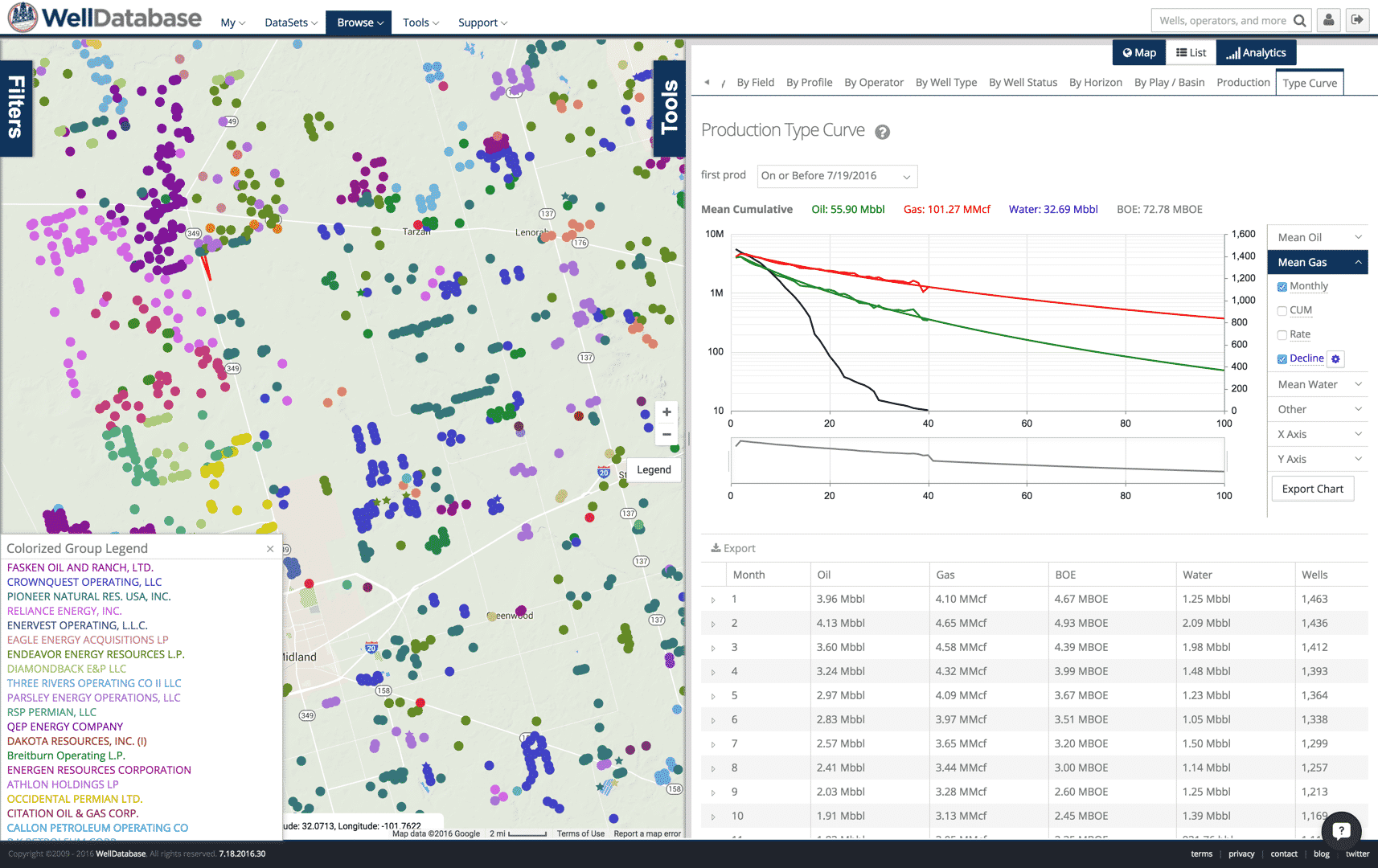
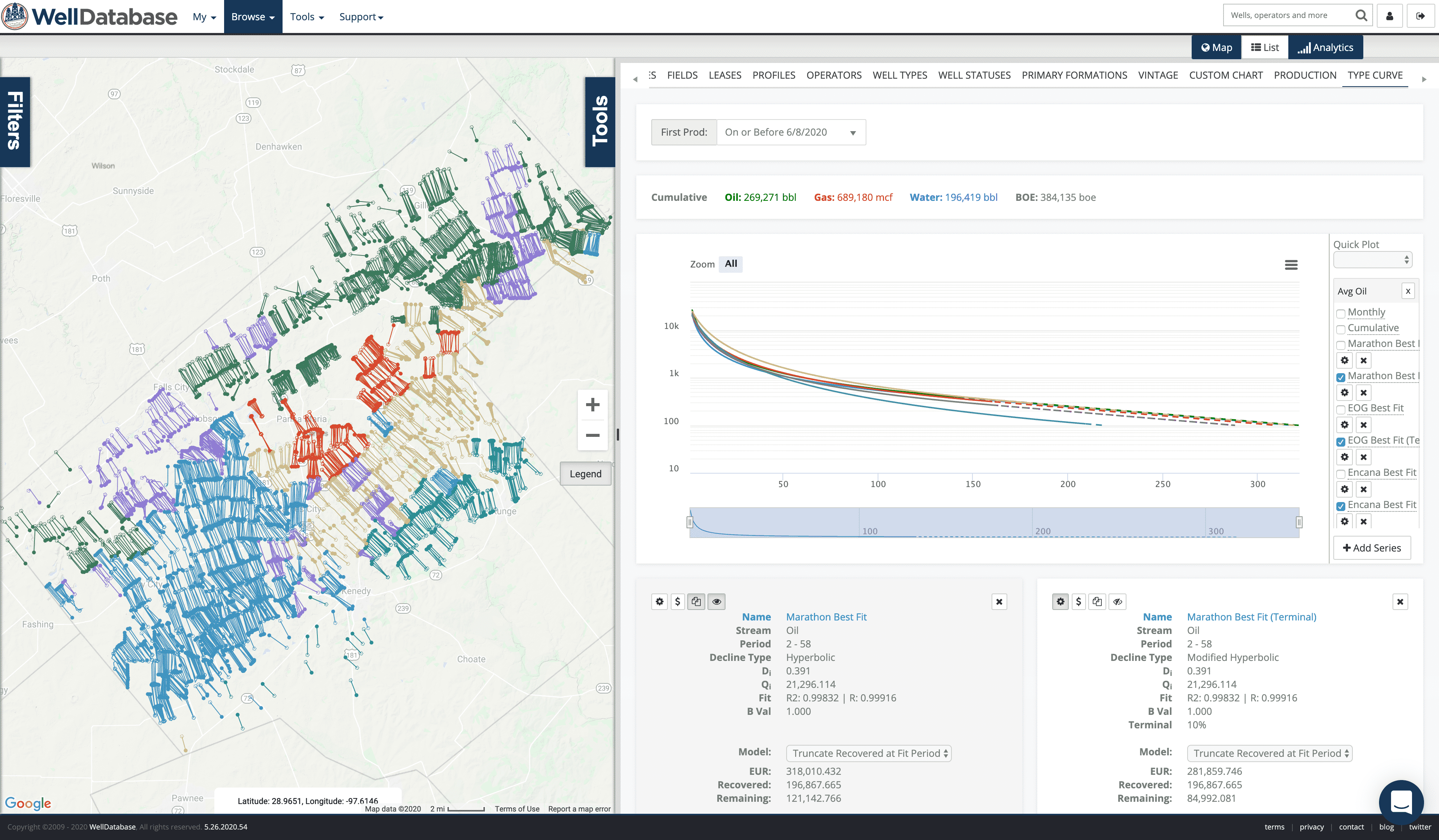
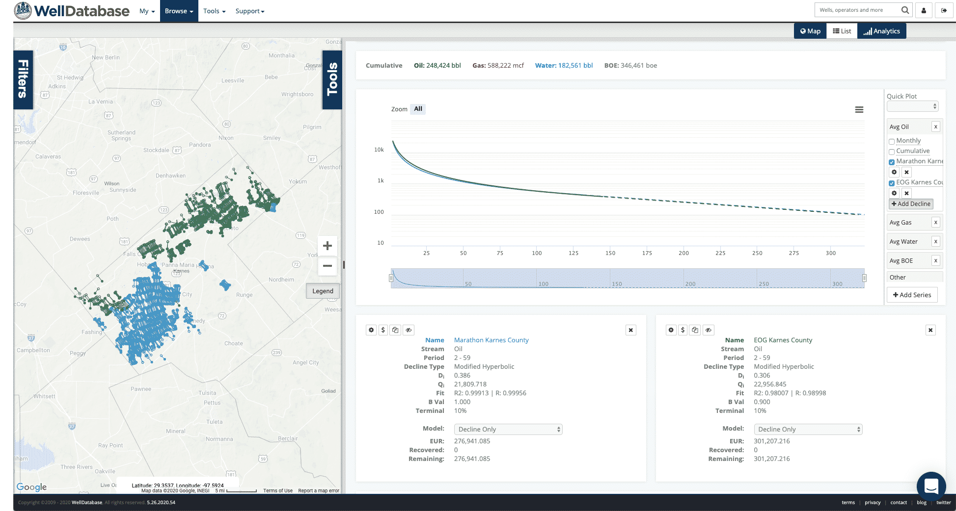
Out of the 2,435,234 ways to use decline curve analysis, one is to compare operators. Comparing the average type curves for each operator based on...
You need data. You need mapping. You need tools to analyze that data. Now you can do everything in a single, easy to use platform.
Perfect for users who need access to basic well level data. If you're only interested in a few wells and currently use state sites, this plan is for you.
The industry didn't start with unconventionals and neither does our data. We cover the full historical dataset across every producing state and province. Don't settle for inferior data, check out our coverage for any state or province you're interested in.


Creating a production decline curve is relatively simple. Creating one that makes sense can be more of a challenge. Fortunately WellDatabase’s best fit decline and forecast function can do the work for you. The output is a math based answer that is highly accurate, consistent, and easy to defend. There are no black boxes at WellDatabase though. Here we will detail the process we use to create this curve.
This step is very basic. First we remove the 0 volume months. Not only from the beginning and end, but also in the middle if they exist. We do this because if a well has a 0 volume month in the middle of other producing months, then it was shut in. For the purposes of fitting a production curve, this month needs to be ignored. That may not seem like a big deal, but it can make a big difference in the outcome. We will then identify the appropriate peak we will use to generate the decline. Our decline tool allows you to choose an initial volume and date if you prefer. Otherwise we pick the highest peak to decline from. That’s it for the prep.
Here is where the magic happens. Not really magic though. Just math. In this step we generate 32 different decline curves using Exponential, Harmonic, and Hyperbolic methods. We iterate though b values ranging from 0 to 3. For more info on the equations used, see http://petrowiki.org/Production_forecasting_decline_curve_analysis. Now that we have run each scenario, we are ready to figure out which one fits the best.
In this step we go through each of the decline curves we have created and compare it to the known values. We use the least squares method to generate the difference and determine the fit. For more info on lease squares, see https://en.wikipedia.org/wiki/Least_squares.
Now that we have determined the best fit equation, we run this equation to predict future values. Our EUR values are based on a total of 20 years. Our decline tool allows you to specify the period of time you would like to forecast.
So the process is very straight-forward. It is also based solely on the math. We calculate every well in the same manner. Therefore the results are consistent and very easy to compare.
If you would like to try our decline tool for yourself, sign up for your account at https://app.welldatabase.com/signup.

1 min read
Out of the 2,435,234 ways to use decline curve analysis, one is to compare operators. Comparing the average type curves for each operator based on...

1 min read
We’ve been hard at work here at WellDatabase. We are constantly updating our platform to provide the best possible tools and data. The latest target...

1 min read
Well vs. Lease/Unit & Where Formation/Pool Splits Are Required (US + Canada + Offshore) Last verified: September 3, 2025