1 min read
What you get with WellDatabase Lite
We rolled out our WellDatabase Lite package a few months ago. The most common question we have gotten is, “What do we get with WellDatabase Lite?”....
You need data. You need mapping. You need tools to analyze that data. Now you can do everything in a single, easy to use platform.
Perfect for users who need access to basic well level data. If you're only interested in a few wells and currently use state sites, this plan is for you.
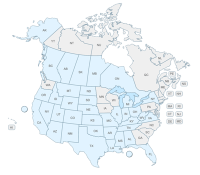
The industry didn't start with unconventionals and neither does our data. We cover the full historical dataset across every producing state and province. Don't settle for inferior data, check out our coverage for any state or province you're interested in.
Now that we’ve released our updated decline curve analysis tools, it’s time to get into the details. The number one question we get is, “What exactly does the best fit do?”. It makes sense, right? You click a button and the curve looks good, but is it? If you are expected to make decisions on this data, you have to know how it’s made. You have to be able to trust it. So let’s start there.
To generate a basic decline curve, we need to determine 3 variables.
Additionally, a modified hyperbolic requires an extra variable, terminal decline rate (Dlim).
At the most basic level, the best fit plugs in values for the variables and tests to see how close it lines up with the actual data. A pretty simple idea for sure. But this blog is all about details.
This part is up to the user. The WellDatabase platform makes selecting a period easy. All you need to do is highlight the range of data you want to use on the chart.
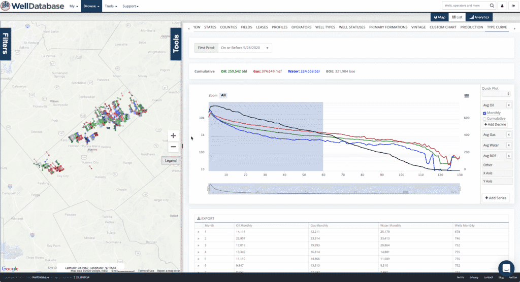
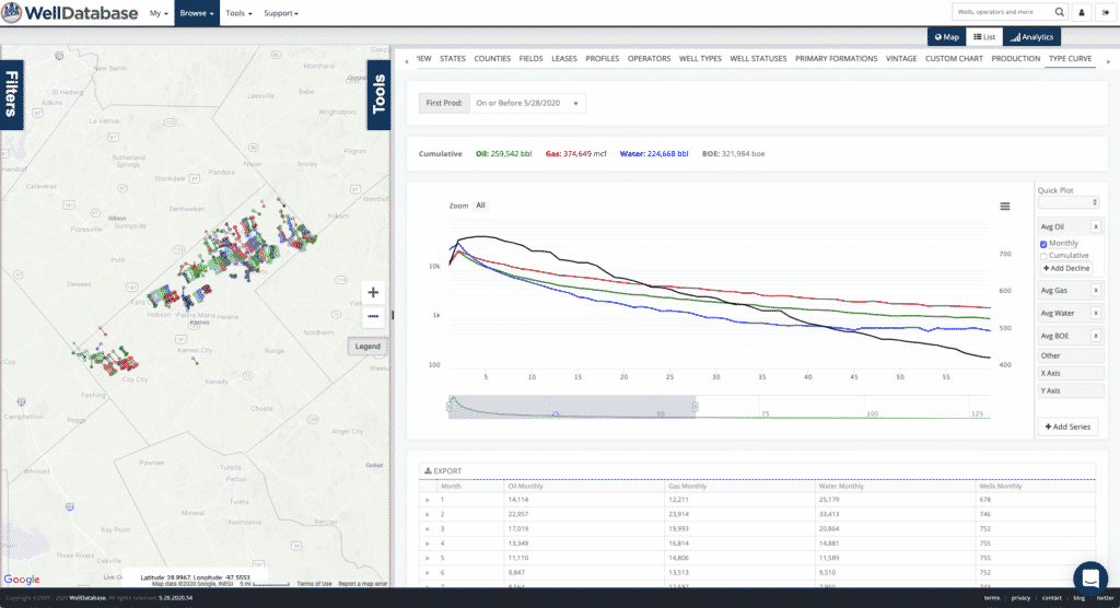
A few quick tips about selecting your fit period.
Feels like we might need an entire blog on identifying the most ideal data set for generating a decline curve. Always making more work for ourselves….
As the “decline” part of the name suggests, we are starting declining in value. So the first step is define where we start. The most obvious choice is the peak value. We use that. Pretty simple idea, but people will change this value at times. The reasoning being that perhaps the max production for a month is not indicative of the actual maximum production period. For our purposes, we don’t care. We stay true to the numbers we have to work with and the max production for the fit period is what we use for the best fit initial rate.
Pro tip – you change the value if you’d like, it just won’t be the best fit.
Now that we have a good initial rate, we need to define the curve for the decline. For those who don’t know the details, the simple idea is this. The initial decline is how steep the values drop and the b value is how curved the line is. Easy enough, right?
Part of the settings for best fit are to choose the range of valid values. Our best fit will loop over these values, create the curve using the parameters, and test the fit to the known data. The default range for B-values are 0-2 and default range for initial decline is 3-90 (it is a percentage decline). You can change these ranges as well and best fit will find the closest fit within that range.
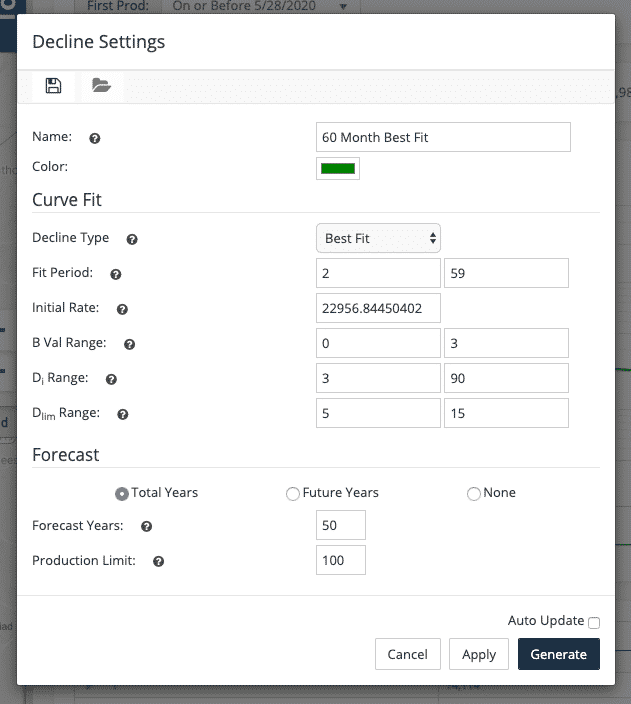
Testing the fit means generating the curve and determining how close the curve values are to the actual values. Decline curves are smooth lines based on an equation, whereas production in real life is much more erratic. The r2 value is what we use to determine how close the values match. The fit will only use the data over the fit period to determine the…fit.
Feels like we’re saying fit a lot. Guess that’s to be expected.
To be precise, we do 2 loops. The first loop is over B-values and the second is over initial decline values. Here’s a couple shots to help illustrate this process.
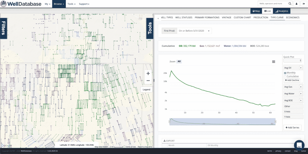
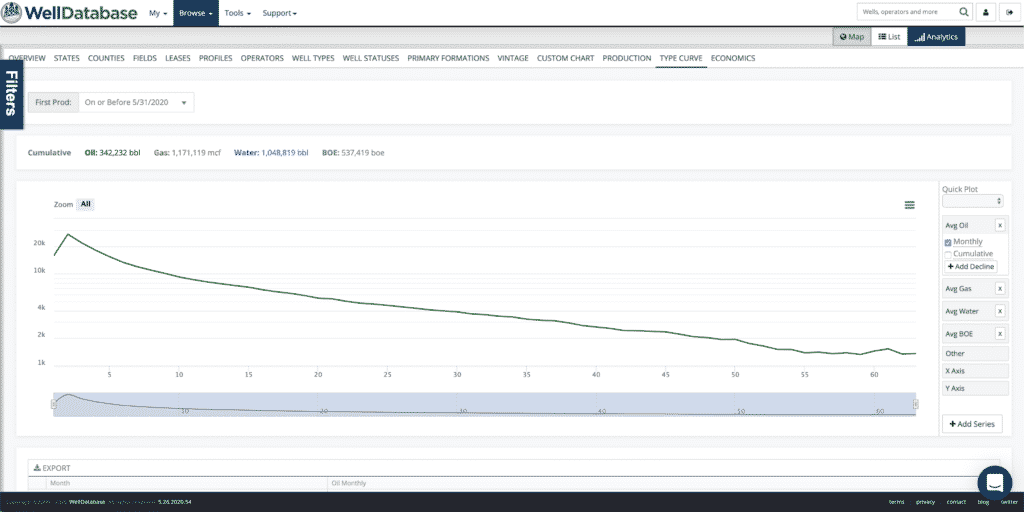
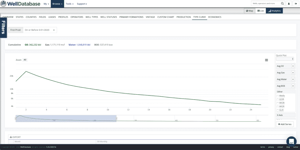
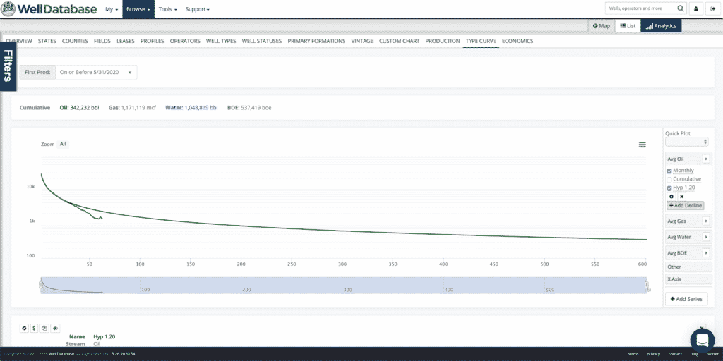
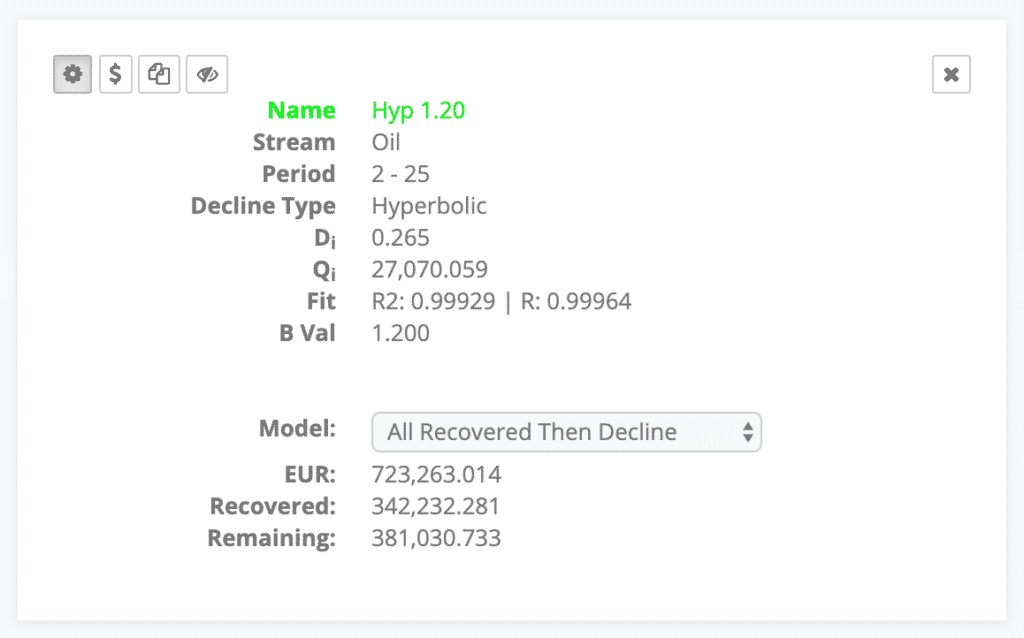
Just for reference, here is the decline summary card for the best fit. You can see that the r2 for the fit is .99929. Also notice that the fit is exceptional over the fit period (months 2-25), but not so much afterwards. This is because the data outside of the selected period is not taken into account when fitting the curve. This particular curve is an aggregated type curve, so we’re fine with that.
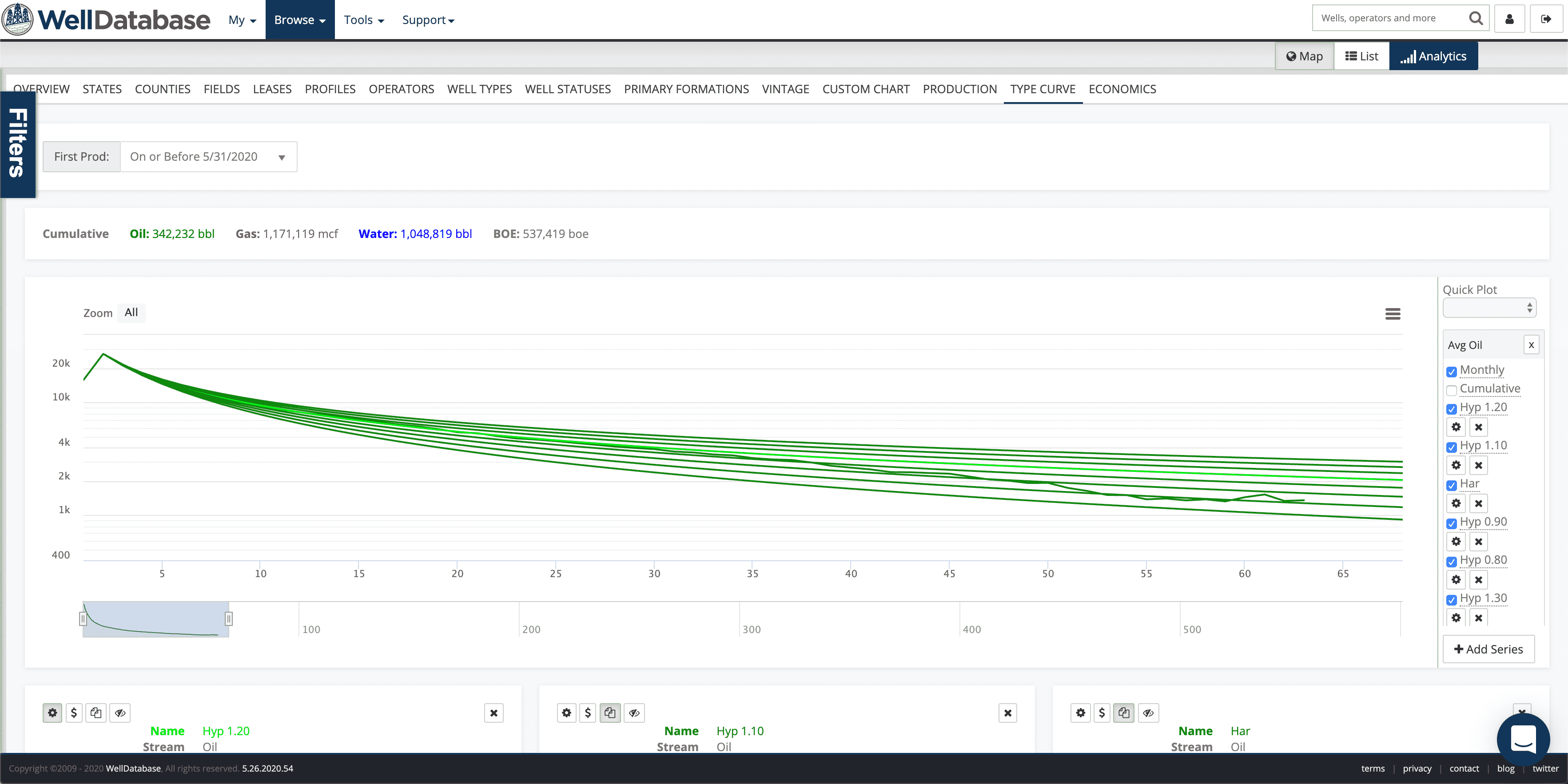
With that best fit in mind, let’s look at just 1 set of parameters we ran. We will plot the 1.2 B-Value, but increment the initial decline values. We made the other scenarios dark green and the best fit light green.
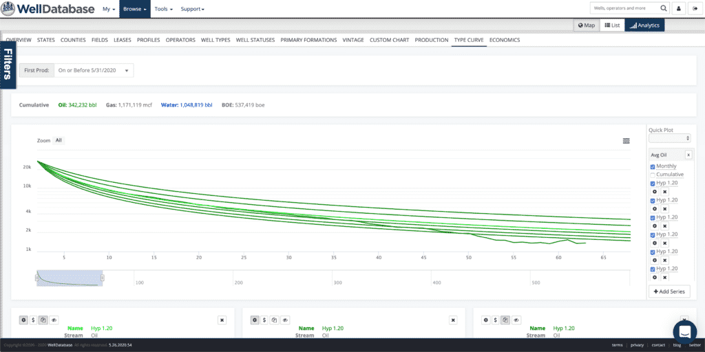
You can see pretty clearly how the initial rate affects the decline curve. Notice that the curvy-ness (technical term) of the line is the same, but the steepness of the drop is different.
Here is a look at the decline cards for each of these. The distribution of EURs on these fits is extreme. We hear a lot about B-values, but the initial decline rate can obviously play a big part in the accuracy of the decline.
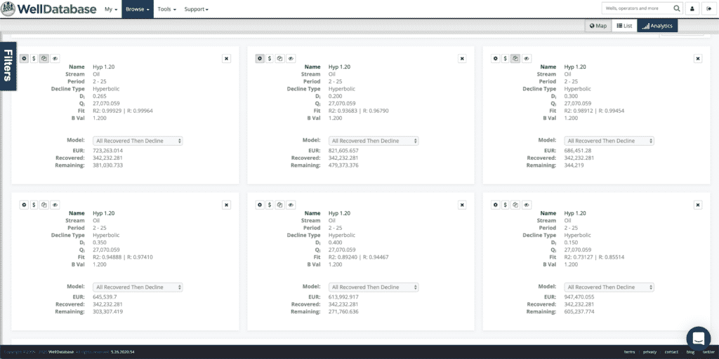
One thing to note about initial decline is that many people just use the difference in the first two months to define the initial decline rate. That sounds a lot like a definition of “initial decline”. While this will get you pretty close most of the time, it rarely is the best fit across the entire curve. It is important to note that the initial decline rate is a parameter that has lasting effects through the life of the forecast. In this case the initial rate for the first two periods is 24.9 and the best fit rate is 26.5. Not a huge difference, but a difference.
Now let’s use that best fit rate and run it over multiple B-values.
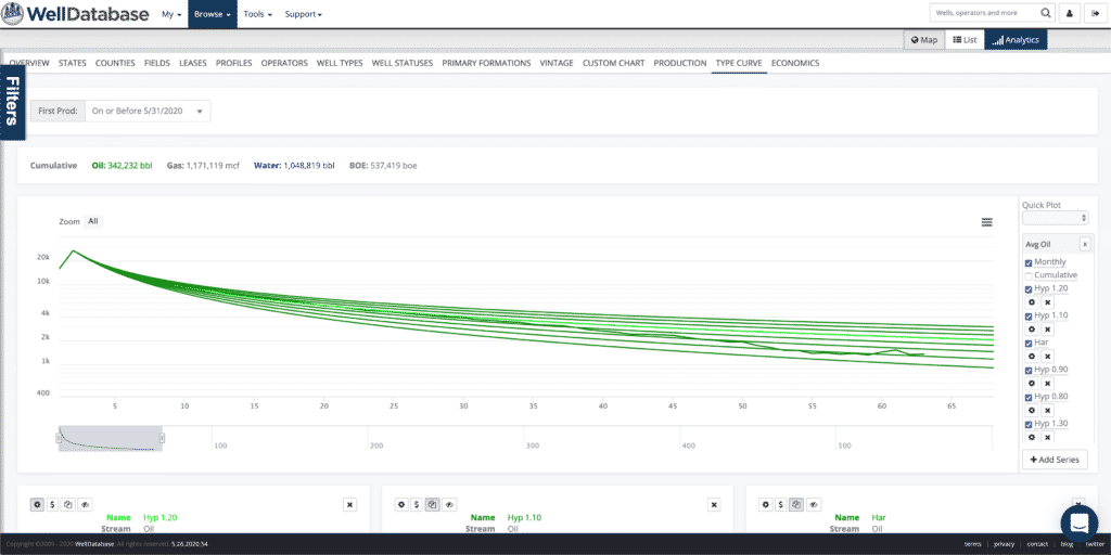
You can see how each of the curves starts at the same rate, but then bends a little different. Higher B-values give a flatter decline and a higher EUR.
Here are the cards for each of these.
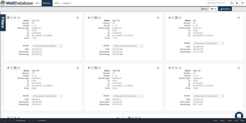
You can see in each of the sets of cards that the r2 for the best fit curve is closer higher than all others. In the set here, the difference in fit between 1.2 and 0.9 is only 0.03734, yet the EUR difference is more than 315k bbls.
As we inch dangerously close to putting you to sleep, we’ll bring this to a close. You can see our best fit is pretty straightforward and grounded in math. Staying true to the numbers is the best way to ensure the fit is accurate and reflects the data.
Hopefully the process is a little more clear. We will follow up with several more blogs around the new decline tools and all you can do with them. Stay tuned.
1 min read
We rolled out our WellDatabase Lite package a few months ago. The most common question we have gotten is, “What do we get with WellDatabase Lite?”....
1 min read
This blog is the latest in our series all about our favorite well identifier, the API number. We talk to a lot of users and we find that there is a...
1 min read
Many have called for M&A for years, and 2020 saw a good amount to aid in consolidation of the industry. It has been busier as of late with $3.4...