Using Decline Curve Analysis to Compare Operators - WellDatabase

Out of the 2,435,234 ways to use decline curve analysis, one is to compare operators. Comparing the average type curves for each operator based on known production is easy. Unfortunately it leaves questions. Some of those can be answered by generating decline curves.

In this example we will look into the top operators in Karnes county, Texas. Karnes is in the heart of the Eagleford play and has a good, established base of wells to work with. We’re also going to focus on oil production. However, this process can be applied on just about any area where you want to rank the operators.

Show me What U Workin’ Wit’

10 points if you get the reference….

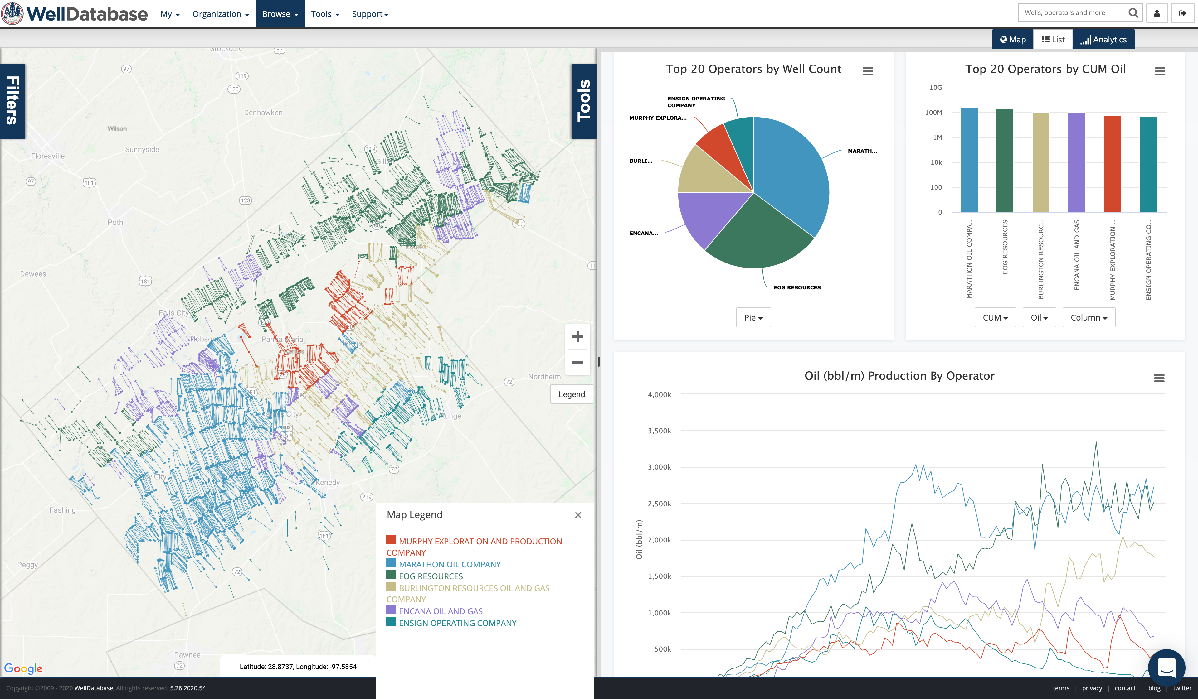
We’ll break down the top 6 operators by well count for wells that came online since 2010. In Karnes county, TX, those operators are:

• Marathon (1,181 wells)
• EOG (874 wells)
• Encana or whatever they’re called these days (462 wells)
• Burlington (Conoco) (371 wells)
• Murphy (247 wells)
• Ensign (221 wells)

Here is the map of those.

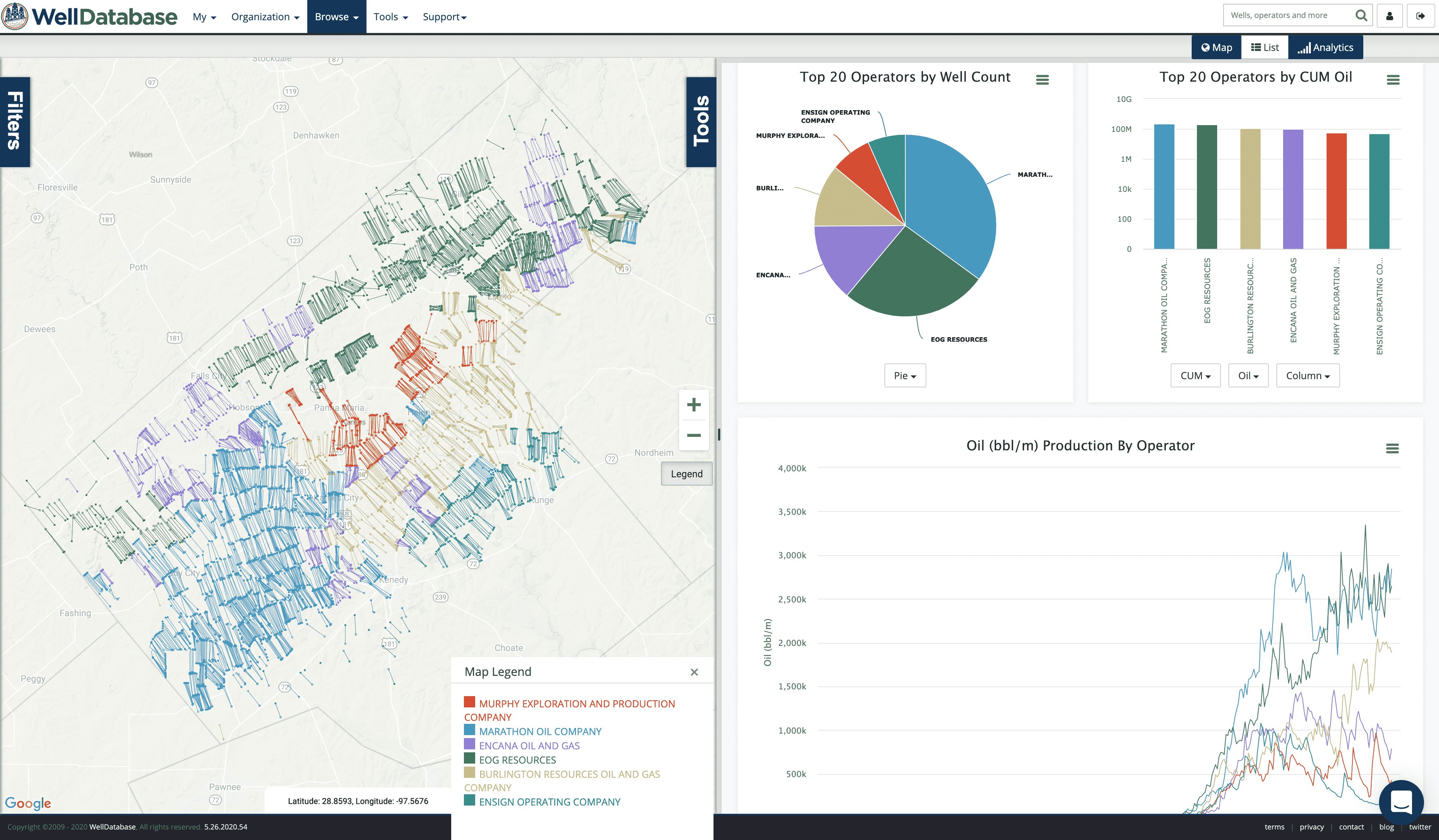
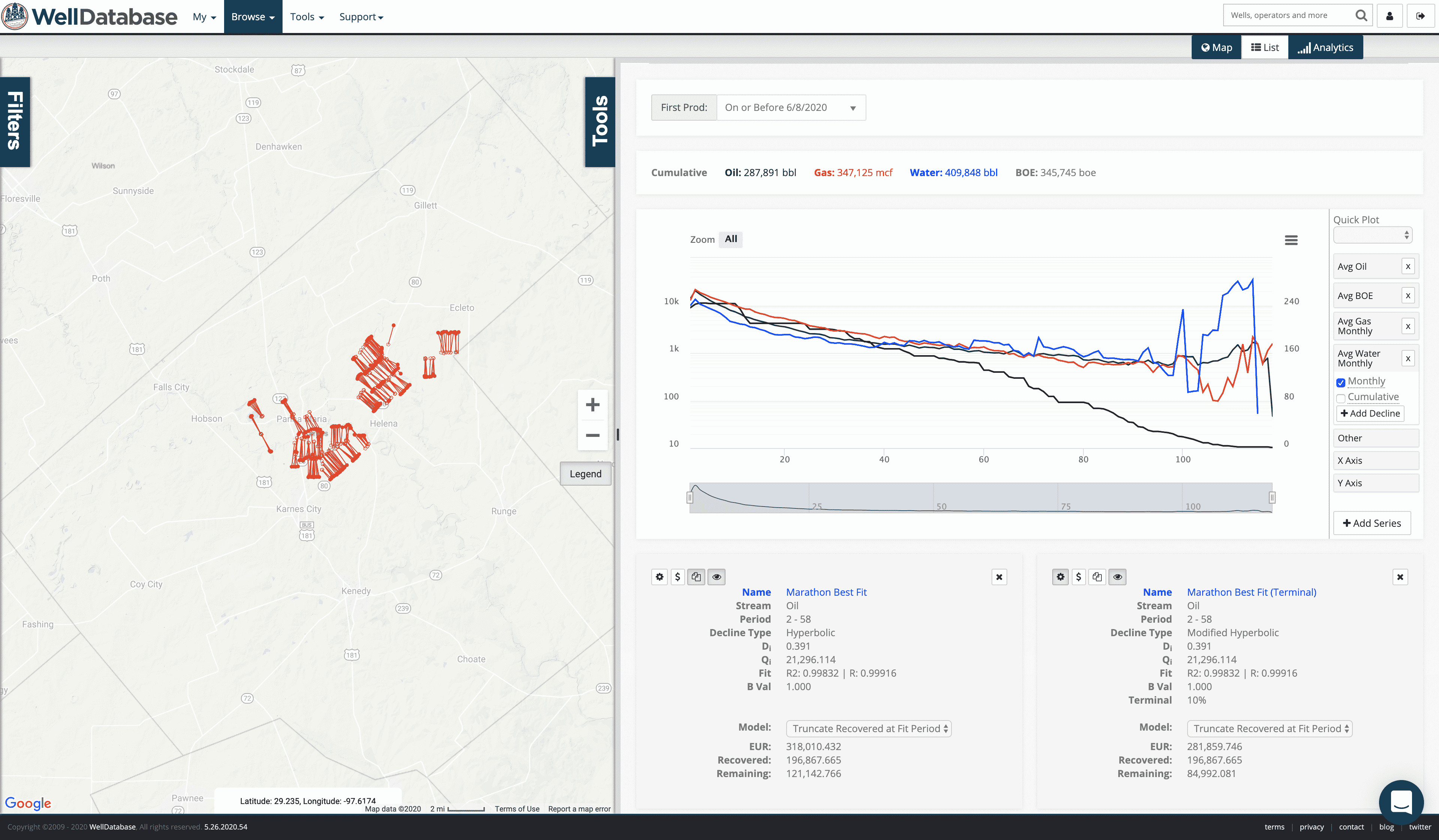
Keep in mind these are wells since 2010. Here is a the screenshot with no date filter.

Since we are comparing production, we’ll stick with wells brought on since 2010.

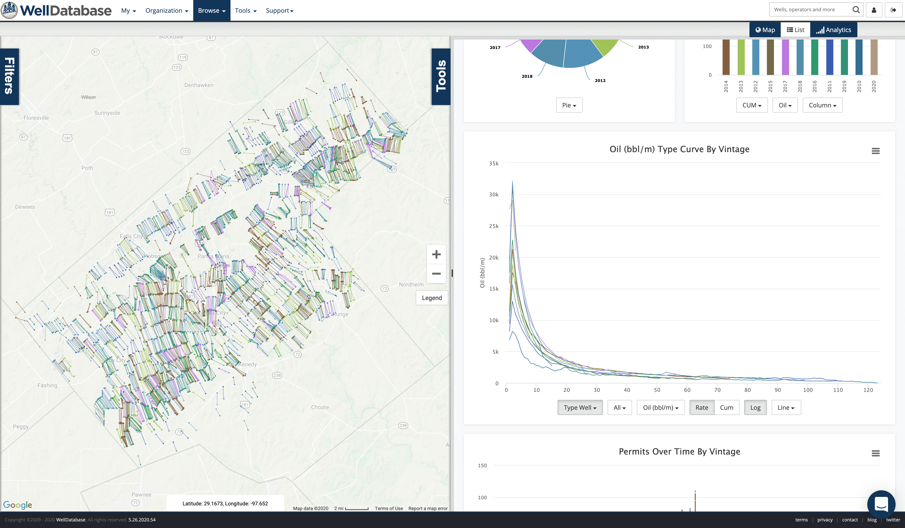
As a side note (something we’ll dive into in a future blog), the type curve changed decently in 2017. Should always keep vintage in mind when comparing operators.

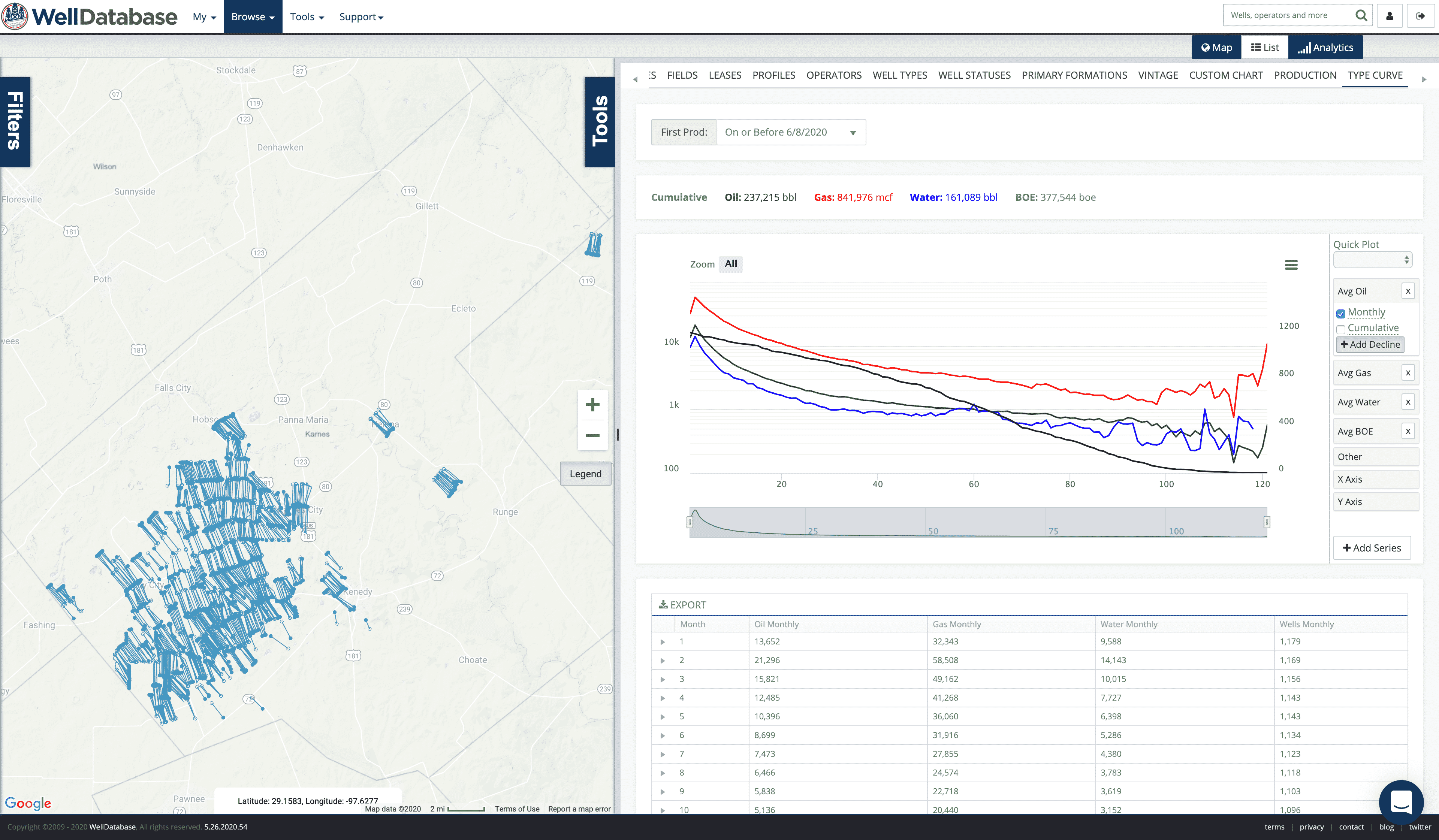
We will be generating a type curve for each operator using our best fit. The fit period will be selected based off the time frame in the type curve where at least 50% of the wells are contributing. Each decline curve will forecast monthly volumes to 50 years or 100 bbls/month, whichever comes sooner. Where terminal decline is not achieved based on the fit period, we will generate a 2nd curve with a 10% terminal number.

Here we go…

Marathon

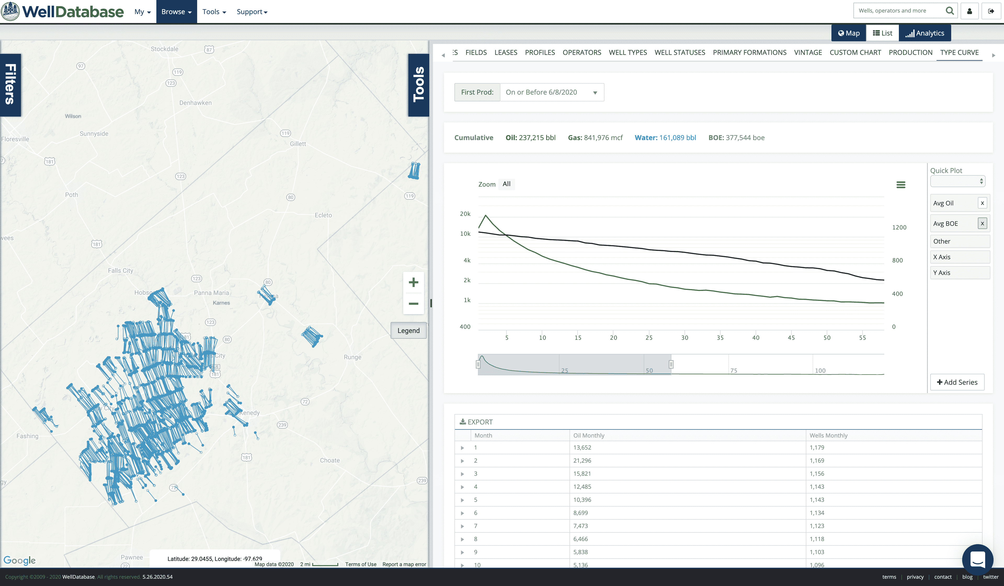
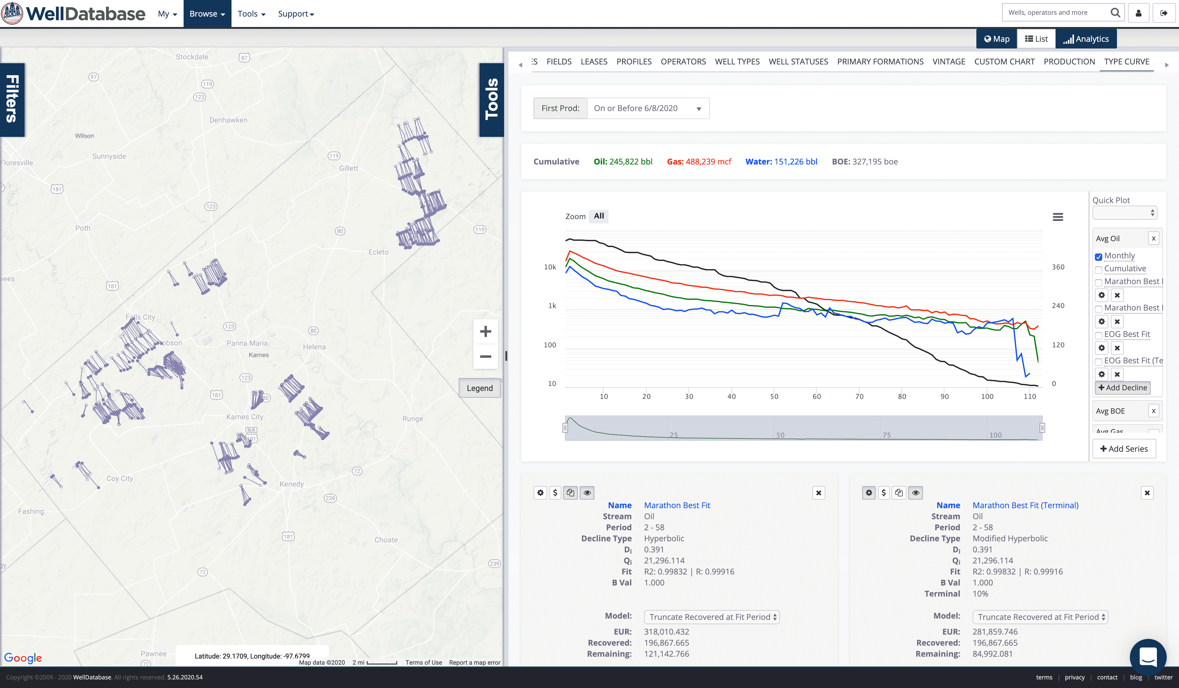
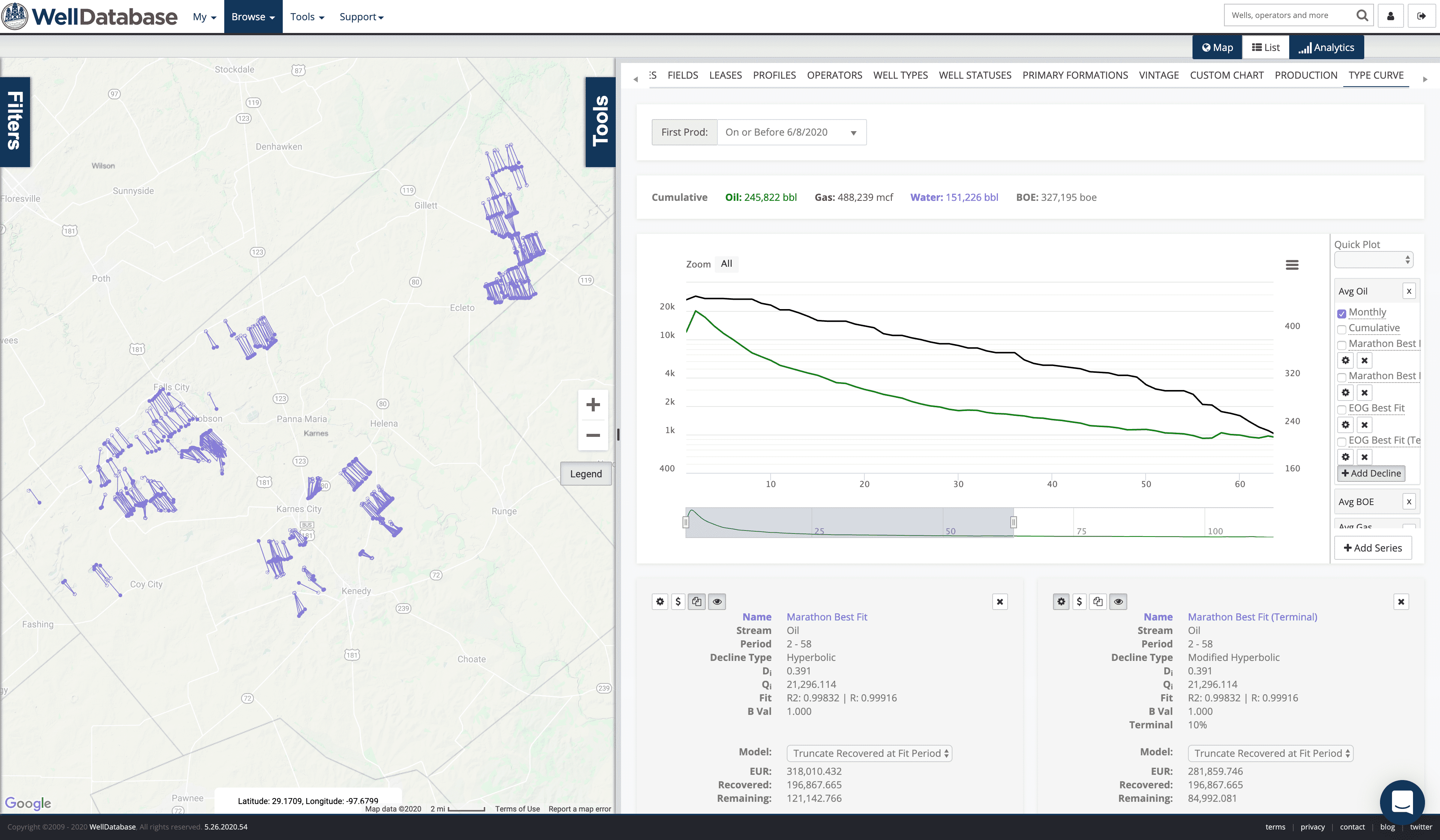
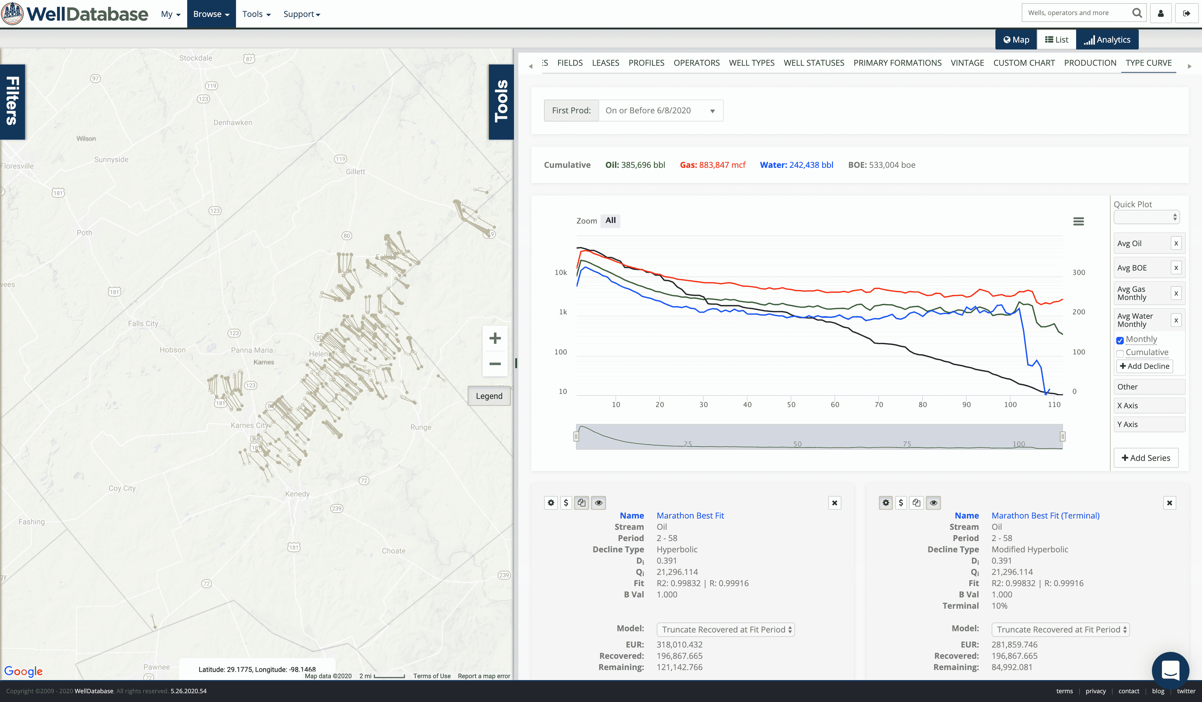
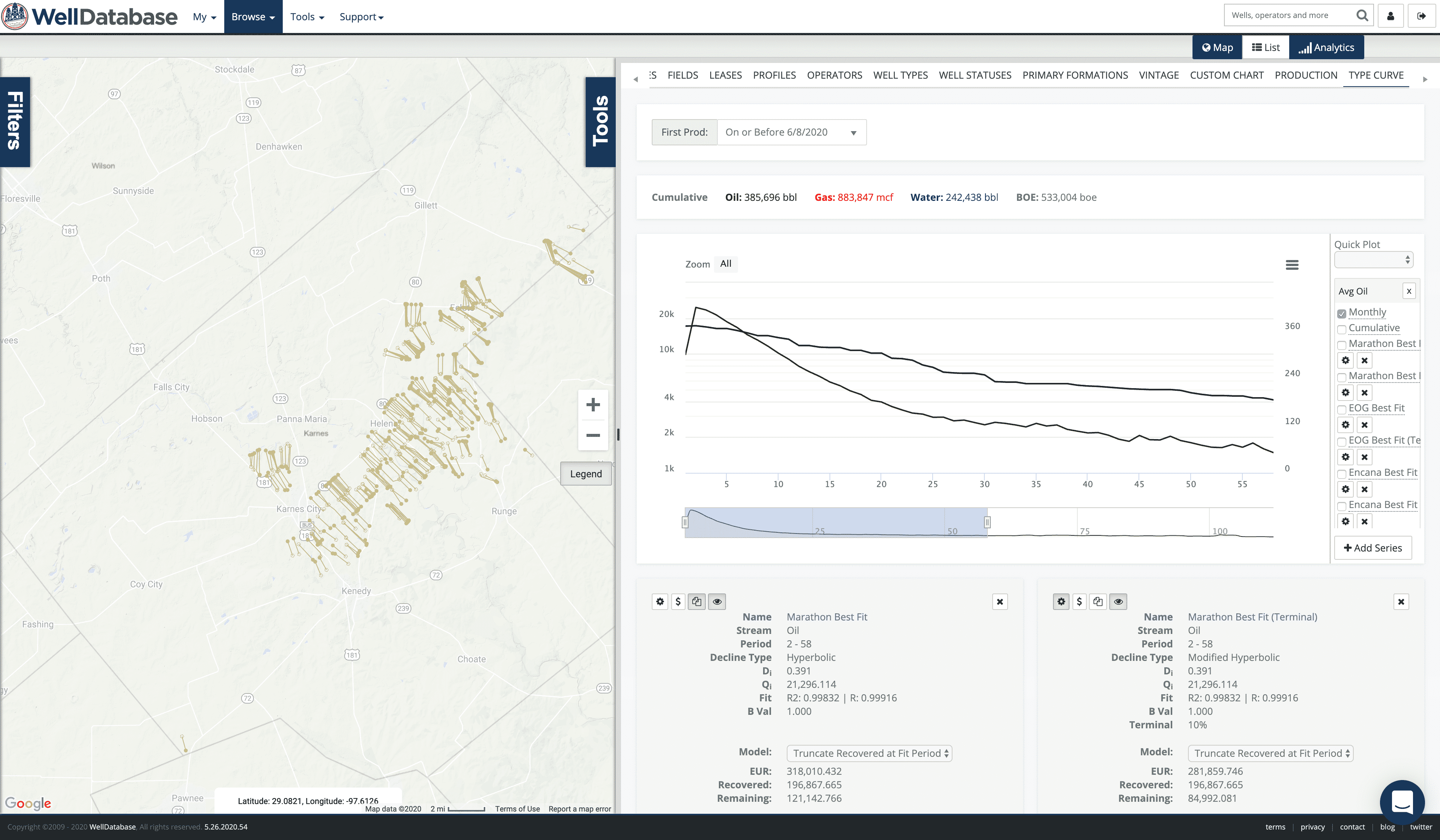
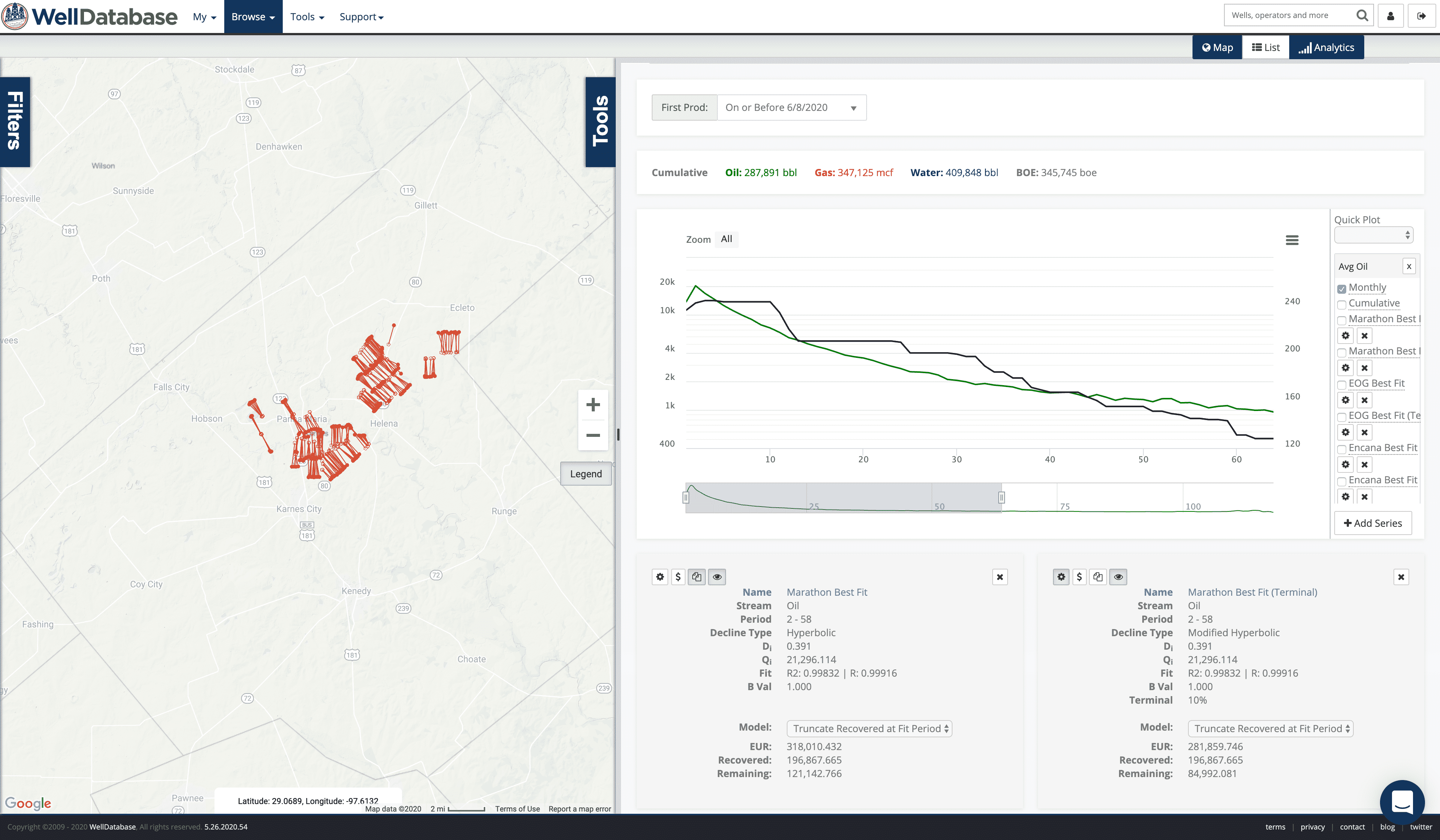
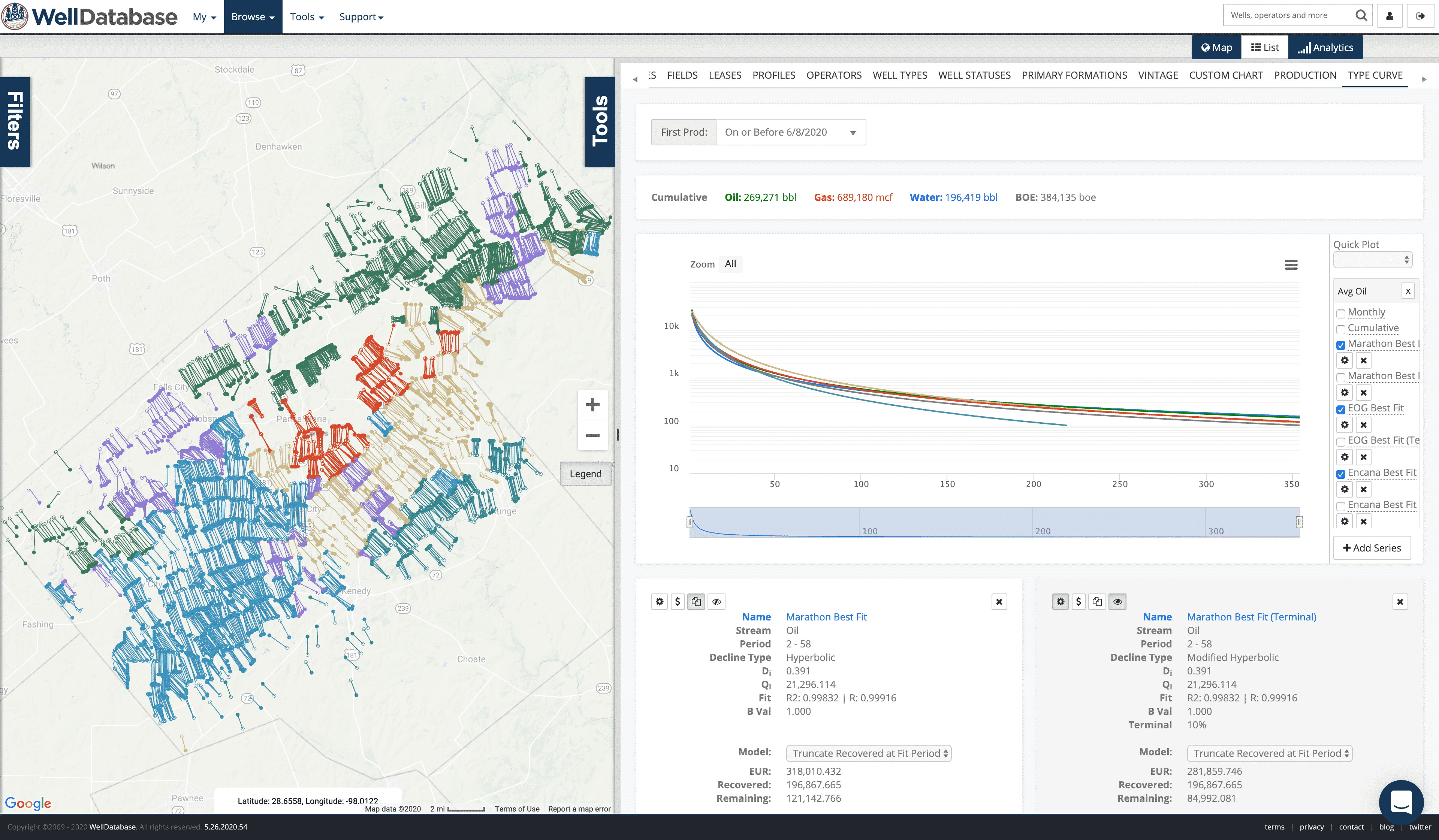
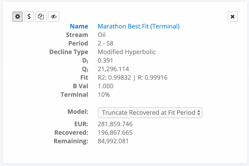
Overall, Marathon’s position and type curves look like this.

The fit period for Marathon is 58 months (600 wells contributing)

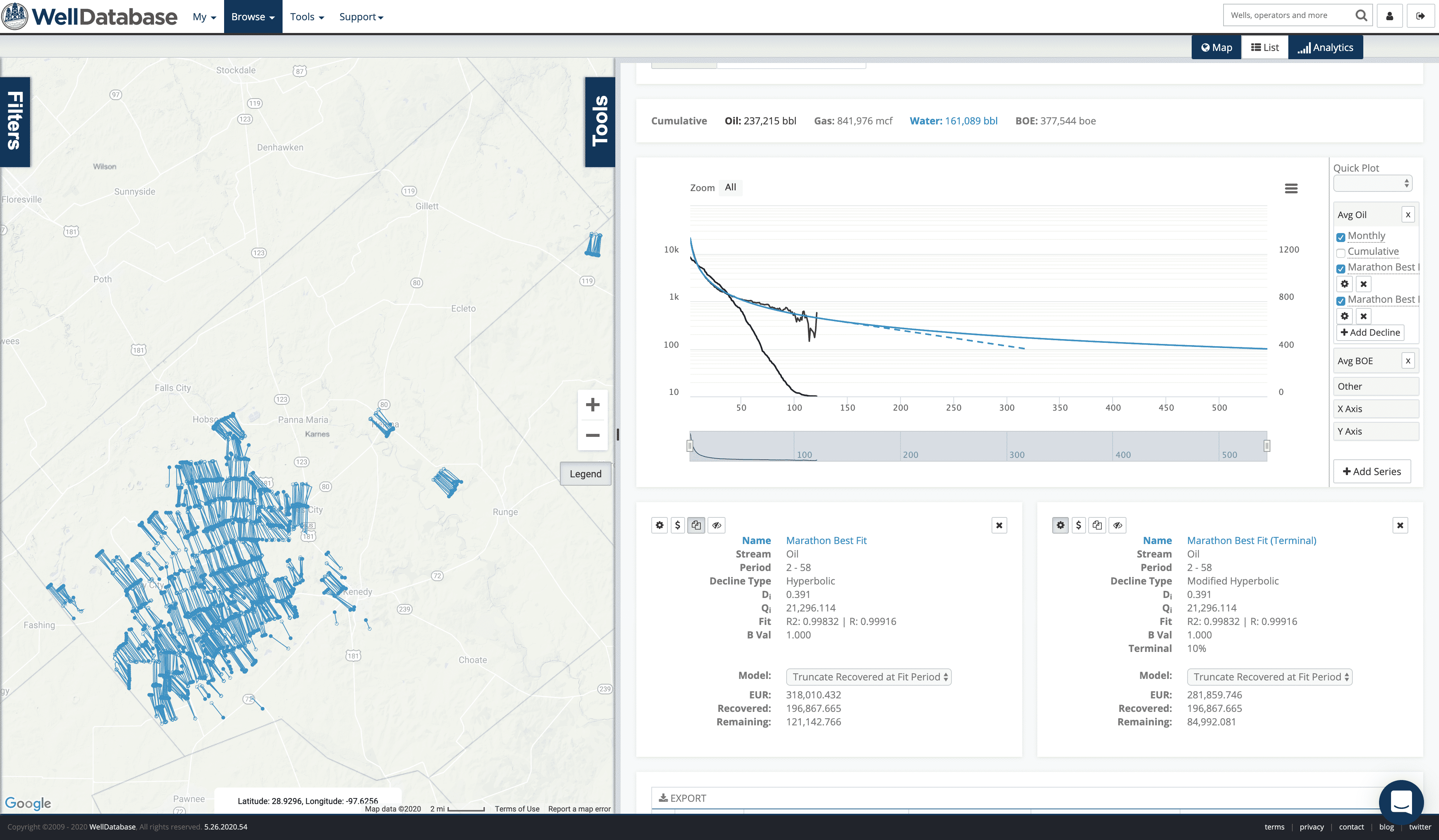
And now the decline. Best fit created curve parameters are:

• Initial Rate – 21,296
• Initial Decline – 0.391
• B Value – 1.0

And like we said, here is the curve with and without a terminal decline.

The difference between the terminal and non-terminal EUR is ~40k bbls. Of course that is achieved with nearly 20 additional years of production. The significance of that is in the eye of the beholder.

We’ll go through the rest of these a little quicker now. Keep in mind we are going to compare these, so we will just be hiding the other company decline curves as we go. You’ll see what I mean.

EOG

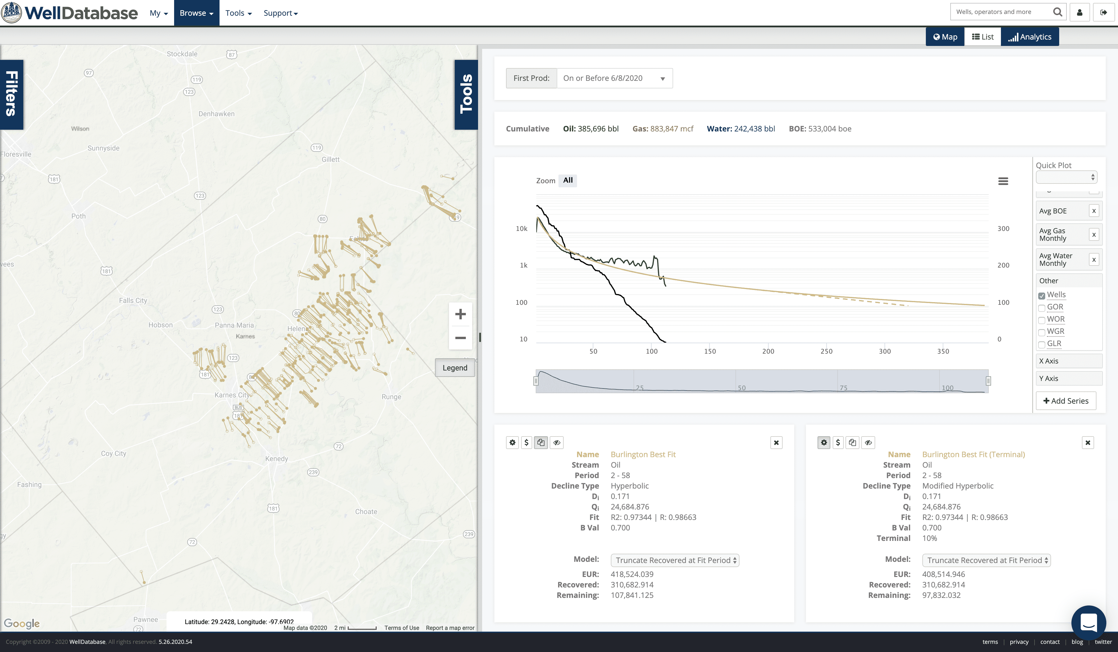
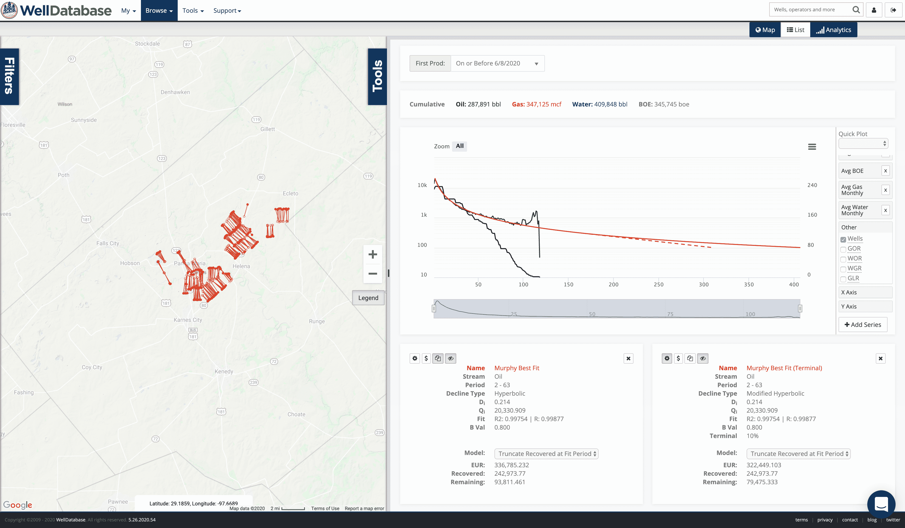
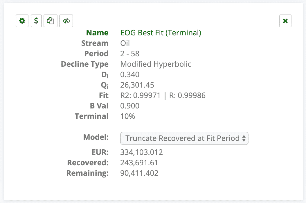
Position and Type Curves.

Another fit period of 58 months

Best fit created curve parameters are:

• Initial Rate – 26,301
• Initial Decline – 0.340
• B Value – 0.9

Encana aka Ovintiv

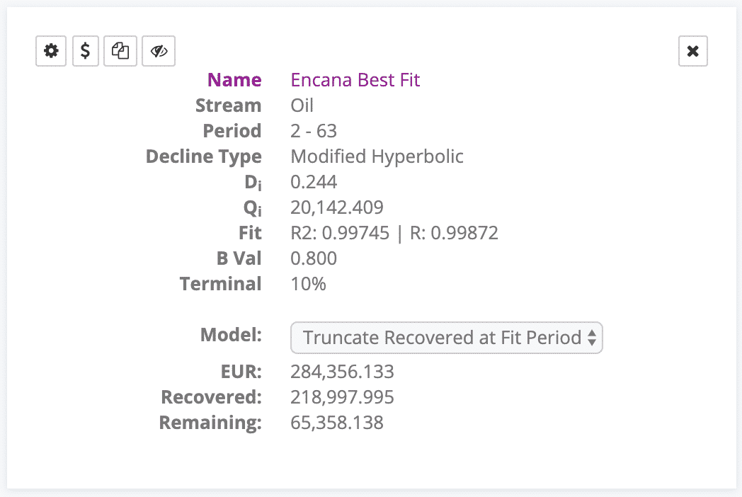
Position and Type Curves

64 months on this fit period

Best fit created curve parameters are:

• Initial Rate – 20,142
• Initial Decline – 0.244
• B Value – 0.8

Burlington aka Conoco

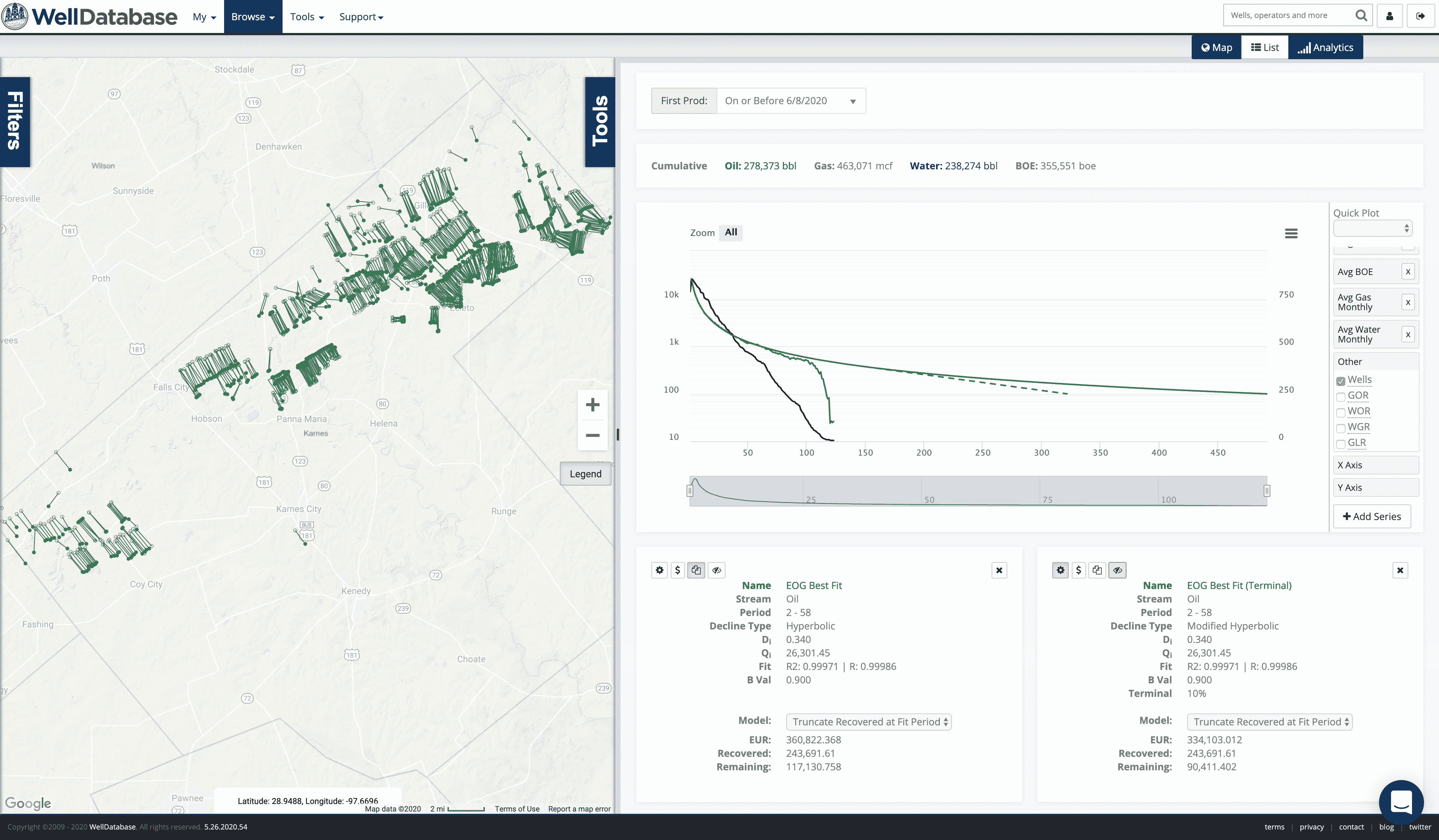
Position and Type Curves

58 months for the fit period

Best fit created curve parameters are:

• Initial Rate – 24,684
• Initial Decline – 0.171
• B Value – 0.7

Murphy

Position and Type Curves

64 months in the fit period

Best fit created curve parameters are:

• Initial Rate – 20,330
• Initial Decline – 0.214
• B Value – 0.8

Ensign

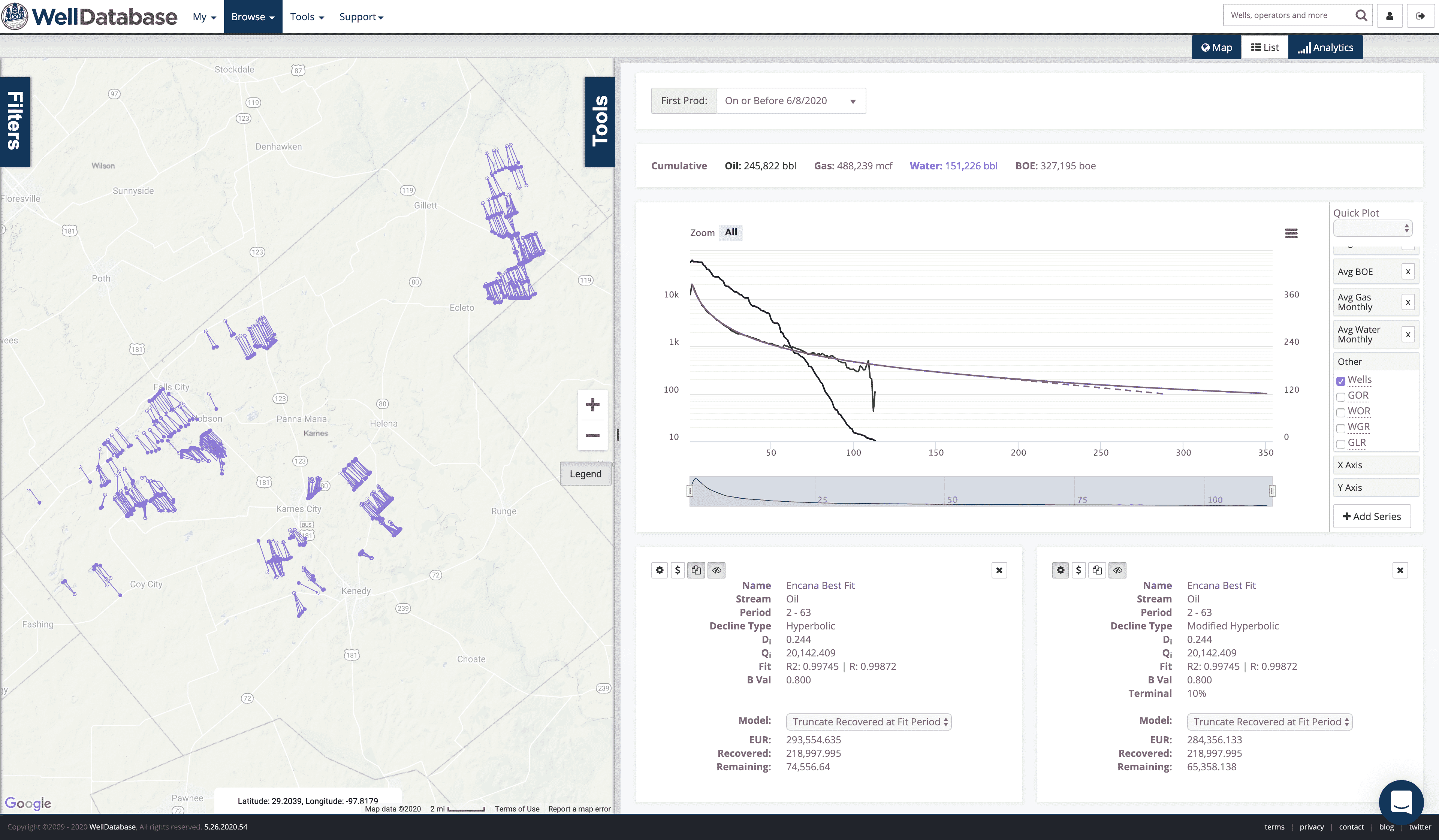
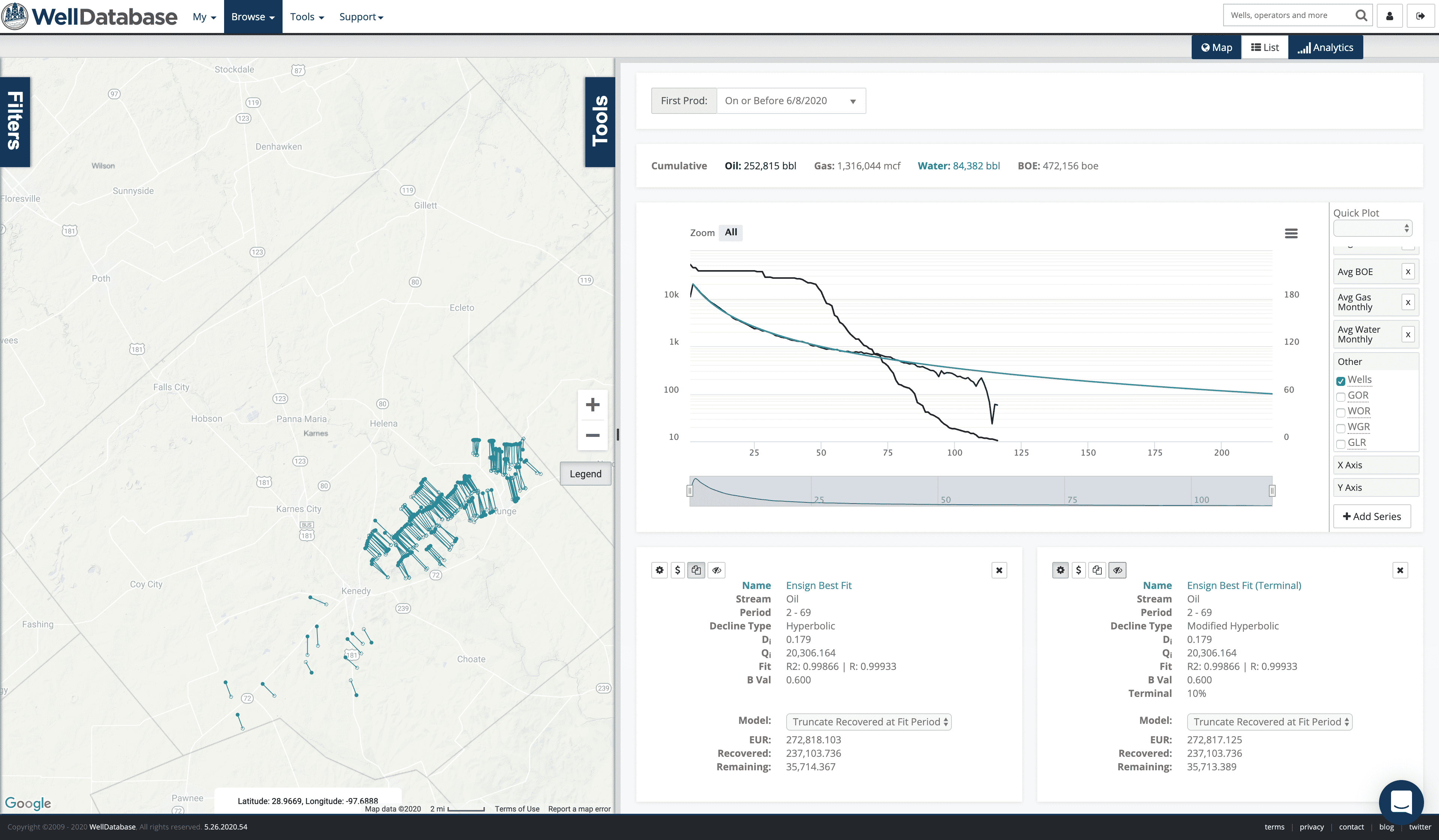
Position and Type Curves

69 months in the fit period

Best fit created curve parameters are:

• Initial Rate – 20,306
• Initial Decline – 0.179
• B Value – 0.6

Together

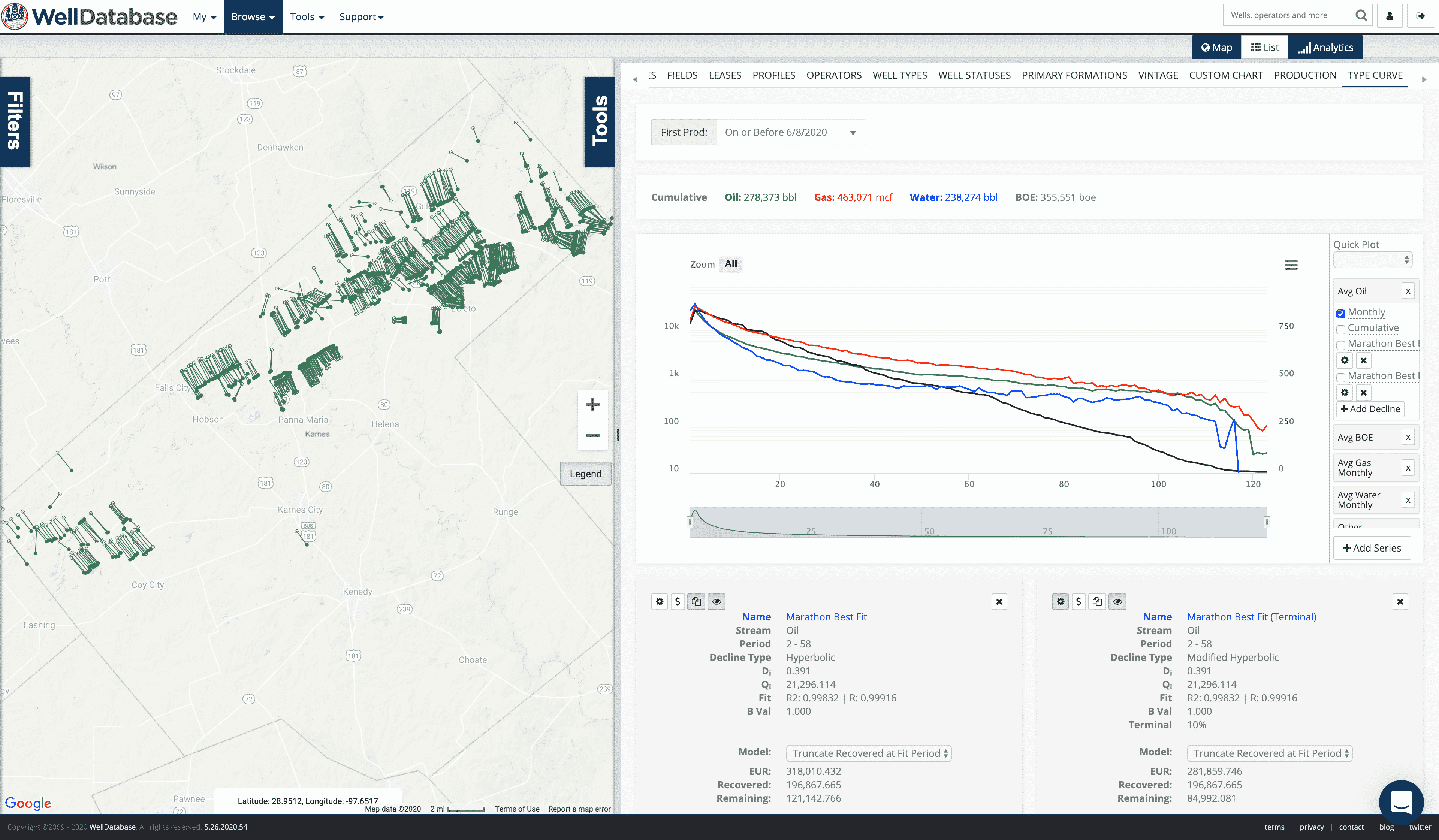
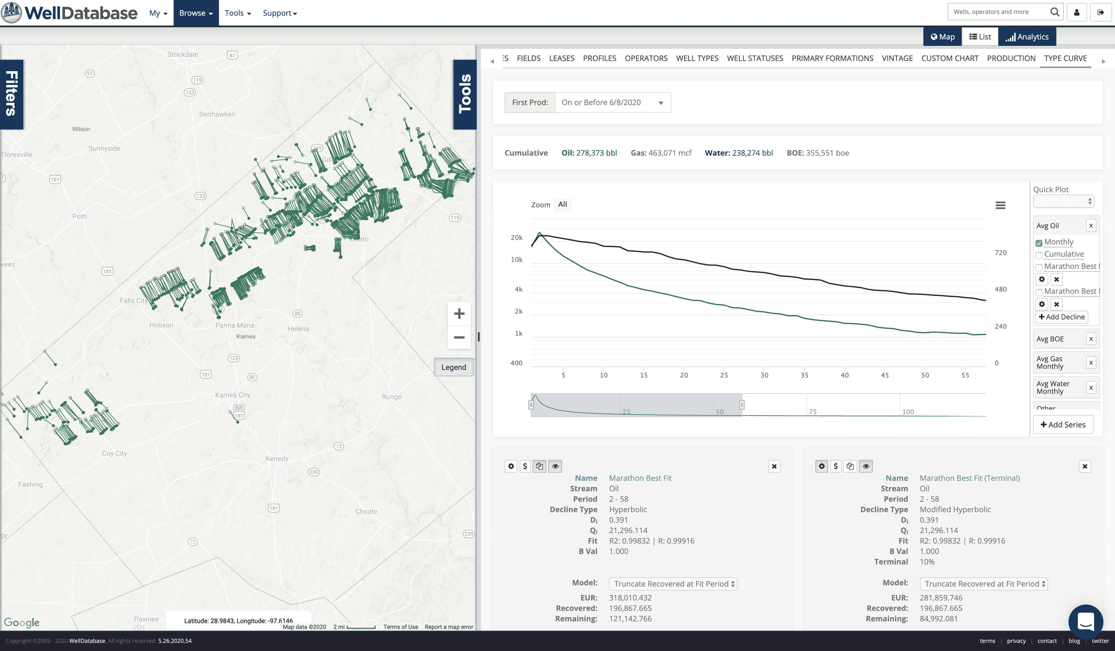
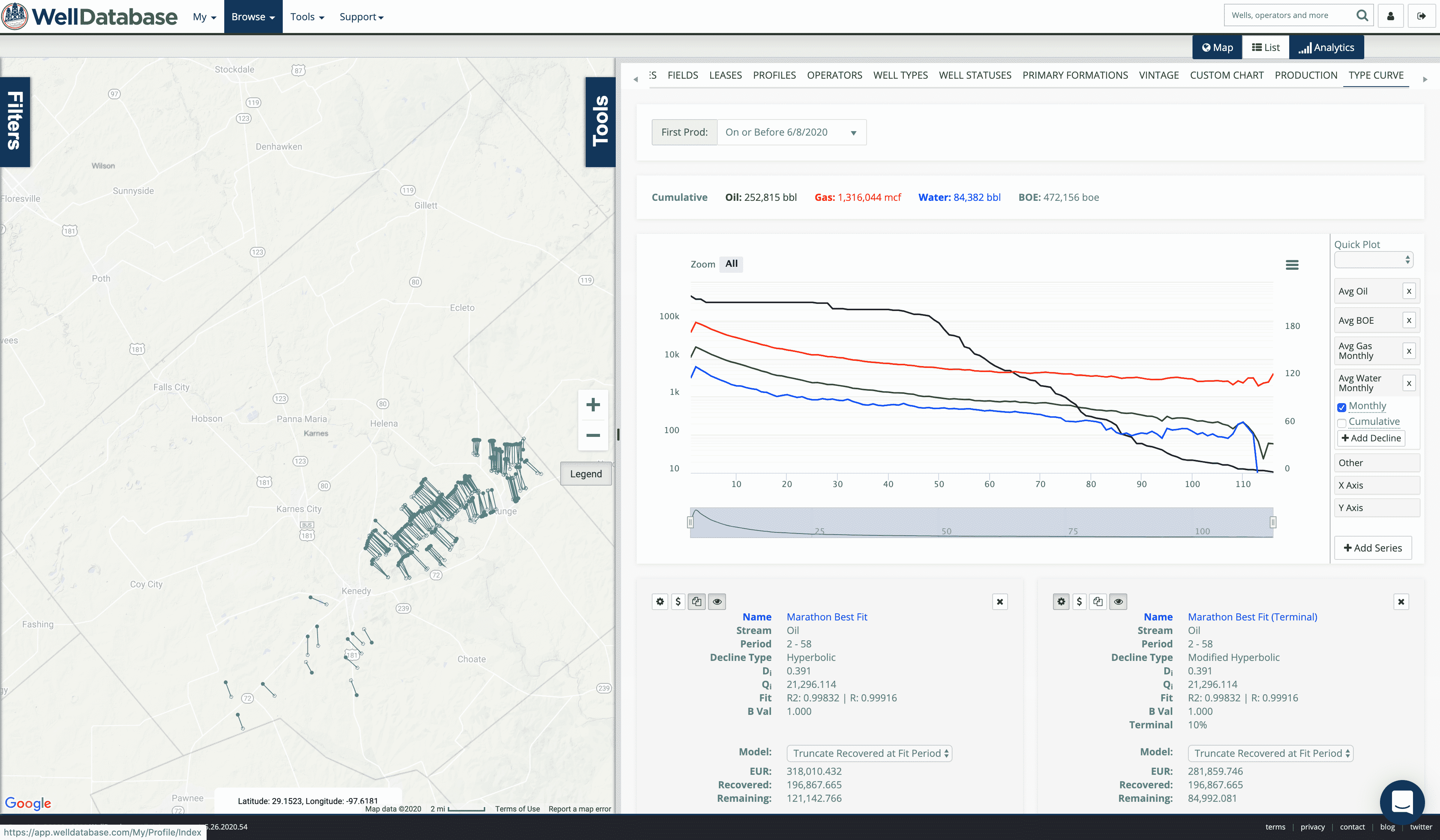
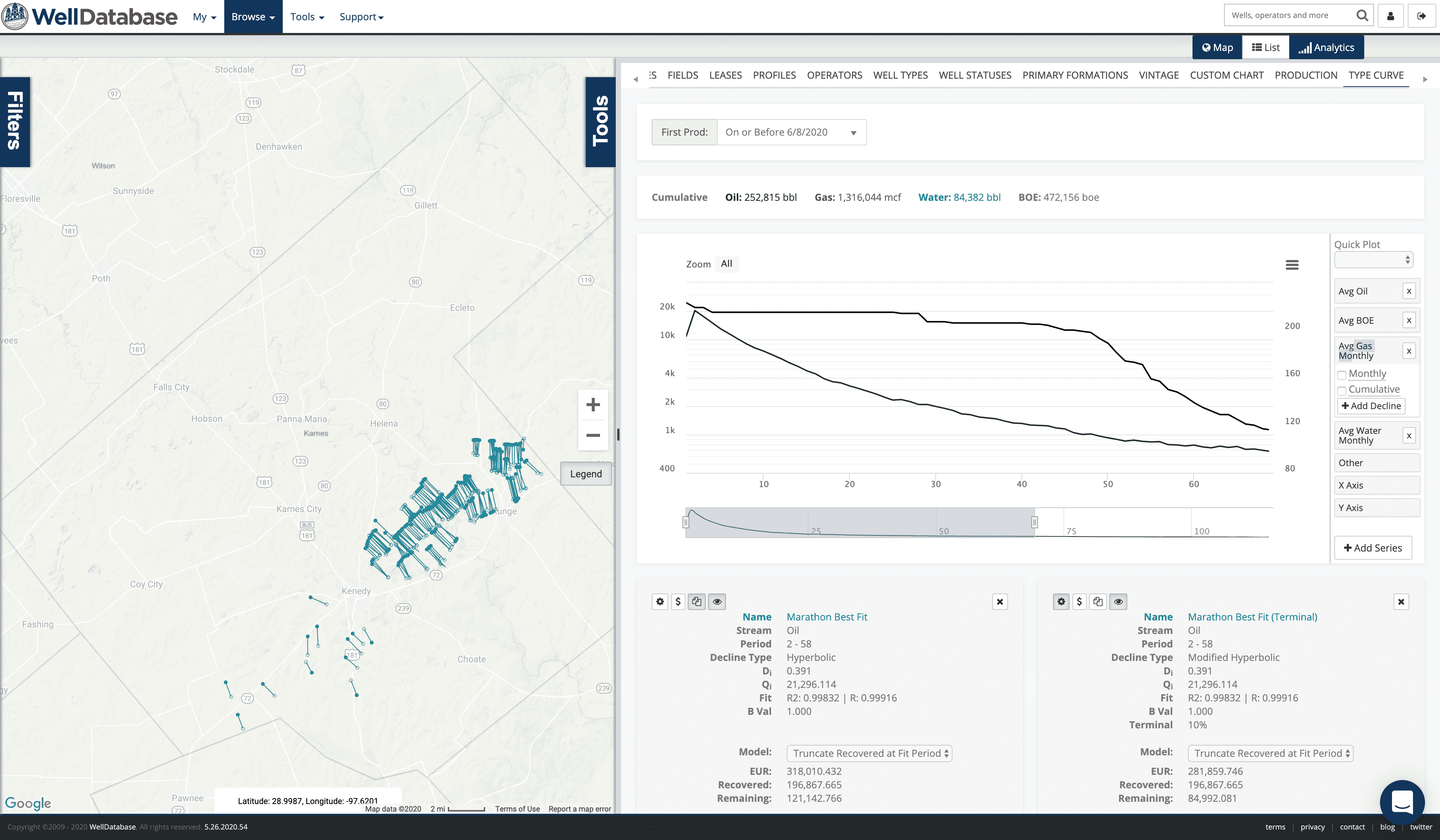
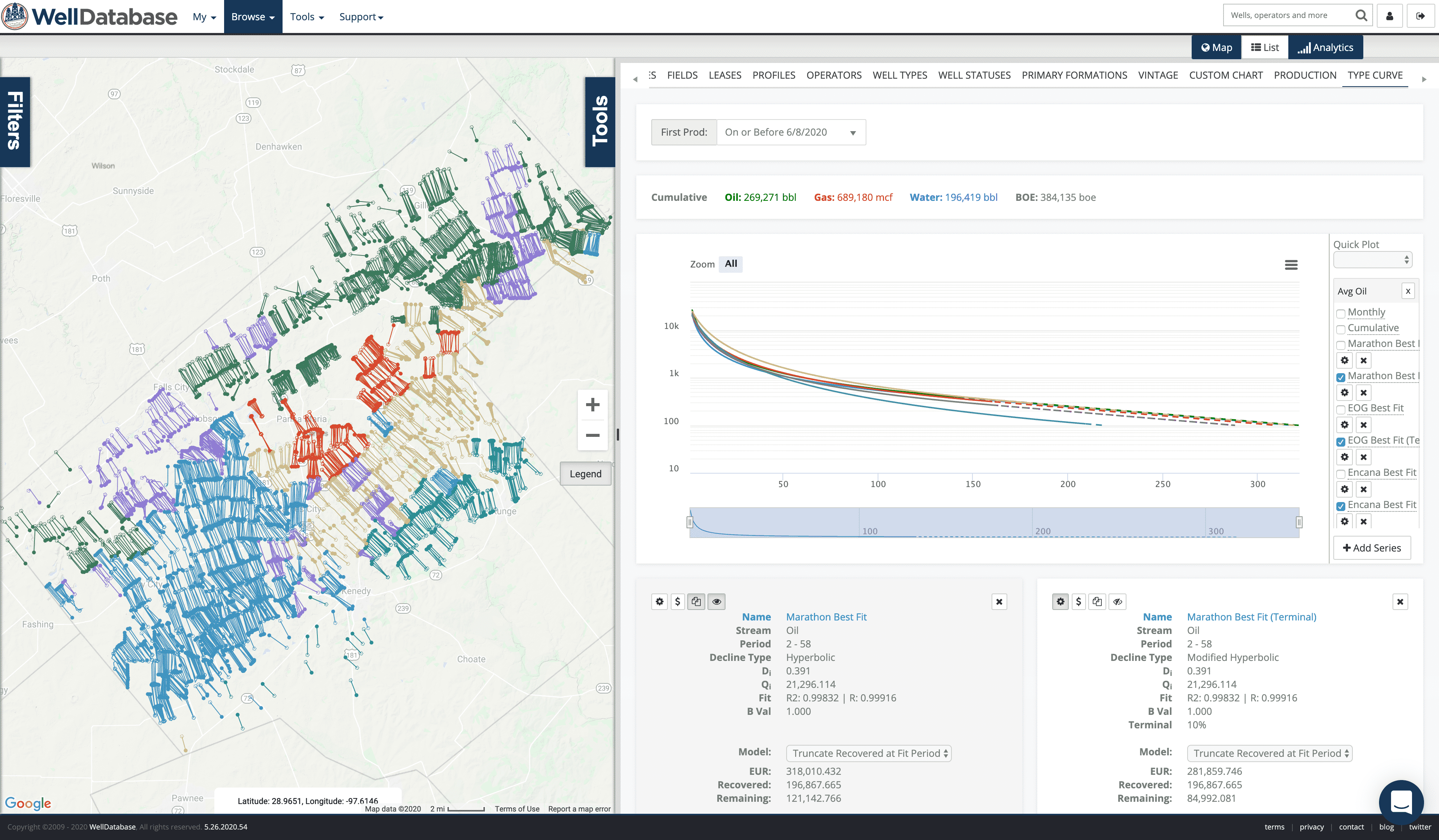
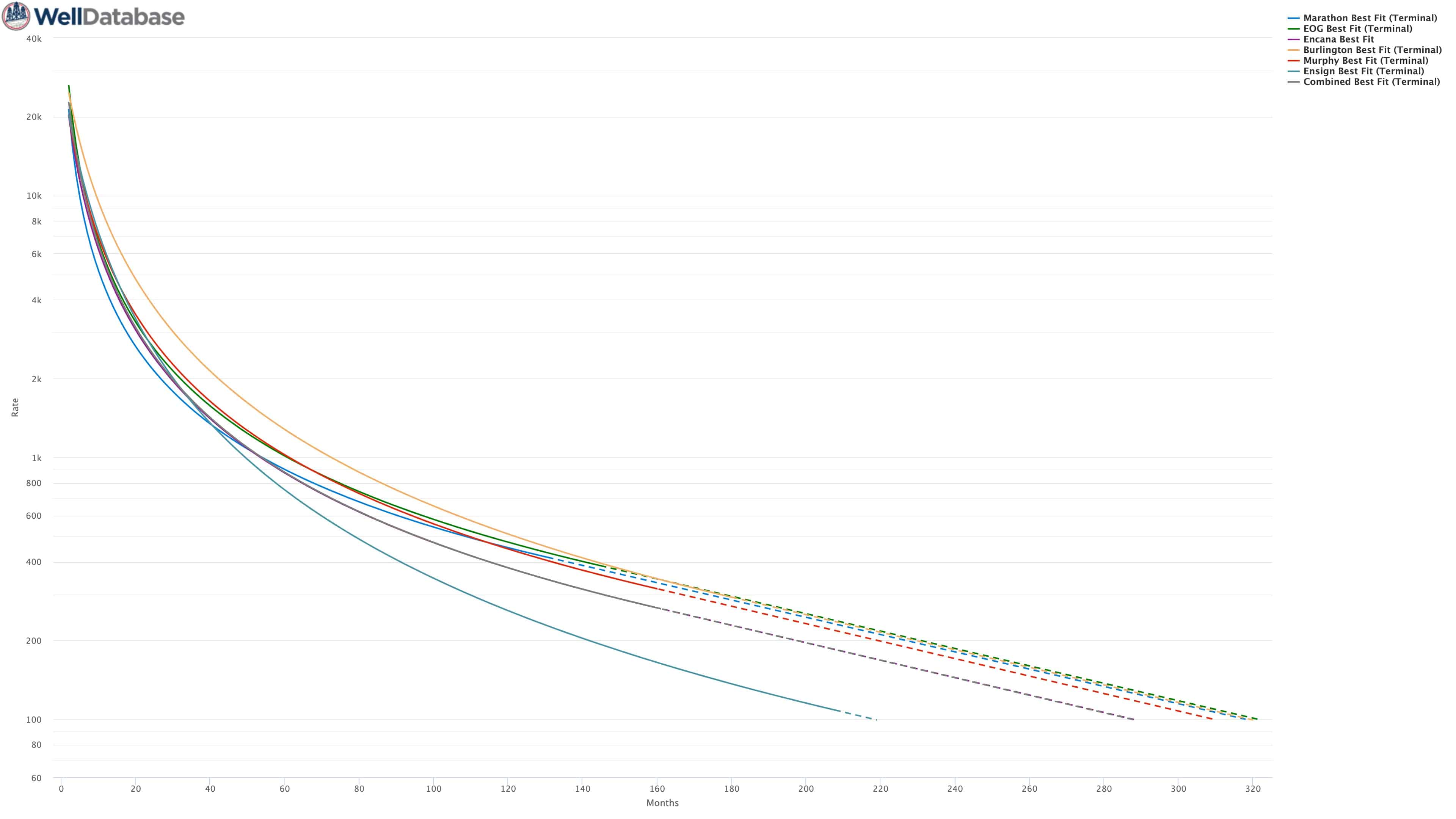
It’s a little messy, but here is what the combined chart looks like for the Best Fit.

And then the Best Fit + Terminal

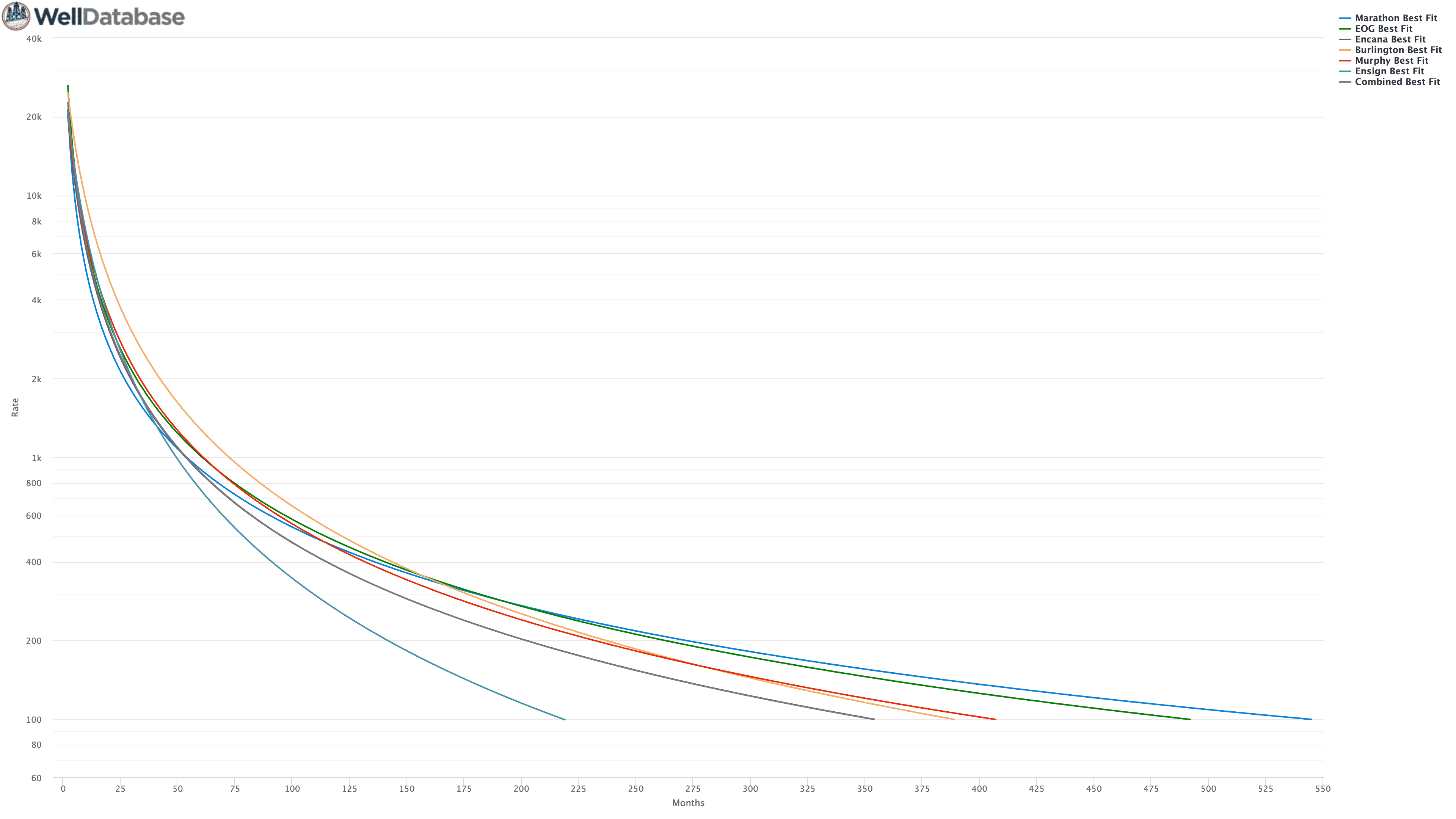
Interacting with the data in this view is useful, but the screenshot is a little hard to read. Fortunately, you can export any chart out of WellDatabase into a hi-res image.

Here’s the Best Fit

And Best Fit + Terminal

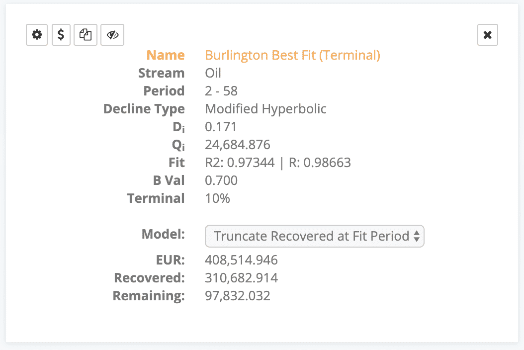
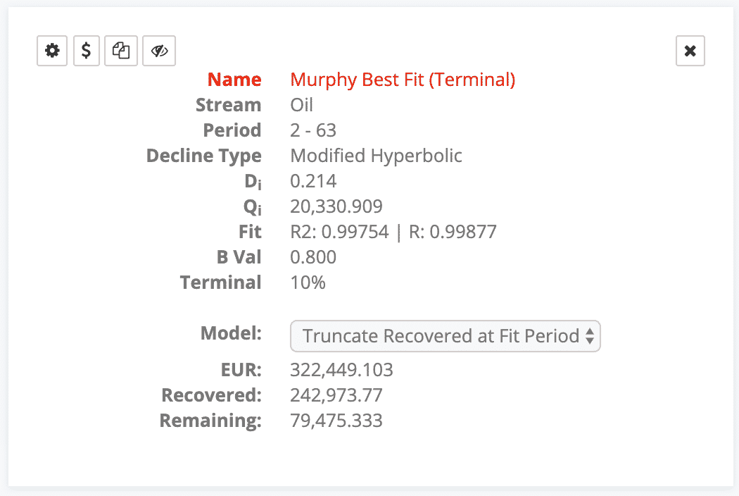
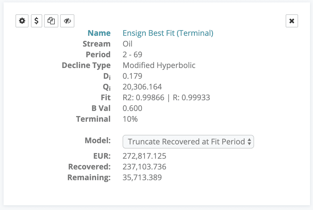
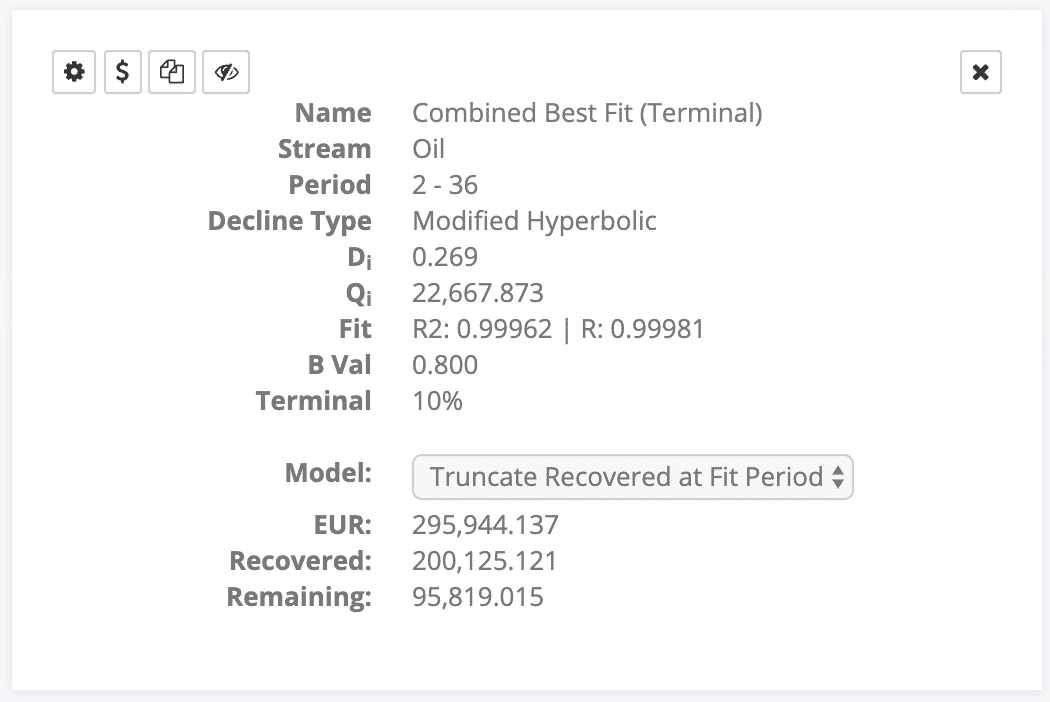
Another useful feature are the DCA summary cards. Here are each of the operator’s cards for the best fit + terminal.

Takeaways

You’ve had to scroll enough already, so we’re going to just lay out some takeaways from this analysis with some simple bullet points.

• Pioneer drilled the Ensign wells. It’s no wonder they wanted to get out.
• The Burlington fit isn’t great. Wanted to leave it as the best fit for this comparison though. Will dive into working with that in a future post.
• The B Value range is 0.6 – 1.0. This is some of the best acreage in the Eagleford. B values > 1 have no business in the Eagleford.
• Karnes county is pretty big (754 mi²). Some variation in production is to be expected. All rock is not created equal.
• Ignoring the Burlington EUR, the range between the best and worst is ~62k bbls.
• Burlington wells have, on average, produced 310k bbls of oil by month 58. That is more than the average EUR for Ensign, Encana, or Marathon.
• I still don’t like the fit or EUR for Burlington though.
• Comparing operators is a challenge. DCA is just one of many tools to do this analysis.
• Marathon wells look like EOG, just without the high IPs. Similar initial decline and b-values. Just ~20% lower initial rate which results in ~20% lower EURs. Math FTW!
• This tool is pretty cool.

If you haven’t tried our new DCA tool, sign up today and check it out for yourself. It is available starting in our Essential package ($250/user/month).